Math 121 - Calculus for Biology I Spring Semester, 2001 Product Rule
	© 2001, All Rights Reserved, SDSU & Joseph M. Mahaffy San Diego State University -- This page last updated 03-May-01

 
1. Sockeye Salmon Populations
2. Ricker's Model
3. Analysis of the Ricker's Model
4. Product Rule
5. Simulation of Ricker's Model
6. Worked Examples
7. Sockeye Salmon of Skeena River Revisited
8. References

The first extension to the study of the Malthusian growth model was the logistic growth model, which improved on the Malthusian growth model by accounting for the crowding effects that result in natural limits to populations. The logistic growth model employs a quadratic updating function, which becomes negative for large populations. Ecologists have modified the logistic growth model in several ways to make the updating function more realistic and better able to handle largely fluctuating populations. One model that is often used in fishery management is Ricker's model. In order to analyze this model, like we have done with the logistic model, the product rule of differentiation is required.

Sockeye Salmon Populations

Recently, the salmon population in the Pacific Northwest has become sufficiently endangered that many salmon spawning runs could become extinct. (This already happened years ago in California.) Salmon are unique in that they breed in very specific fresh water lakes and die. Their offspring migrate a tortuous path to the ocean, where they mature for about 4-5 years. Then an unknown urge causes the mature salmon to migrate at the same time to return to the exact same lake or river bed where they hatched 4-5 years earlier. The adult salmon breed and die with their bodies providing many essential nutrients that nourish the stream where their young will repeat this process. Human activity from damming rivers to forestry, which allows the water to become too warm, to agriculture, which results in runoff pollution, all adversely affect this complex life cycle of the salmon. Many of the ancient salmon runs have now gone extinct.

This life cycle of the salmon is a clear example of a complex discrete dynamical system. Because of the importance of this fish to many people in the Pacific Northwest, there have been many studies of the salmon populations. Below is a table listing four year averages of the sockeye salmon (Oncorhynchus nerka) in the Skeena river system in British Columbia from 1908 to 1952. (The Canadian river systems have not been as severely affected by other human activities as the ones in the U.S.) The table lists the four year averages from the starting year of the data being averaged. Since it is 4 and 5 year old salmon that spawn, each grouping of 4 years is a rough approximation of the offspring of the previous 4 year average of salmon. (It is complicated because the salmon have adapted to have either 4 or 5 year old mature adults spawn, but this will be ignored in our modeling efforts.)

Four Year Averages of Skeena River Sockeye Salmon

We want to use these data to create a discrete dynamical system to describe the population of salmon in the Skeena river watershed. This system can be analyzed to determine information about expected salmon runs to study the health of the ecosystem.

Ricker's Model

We have studied the logistic growth model, which was an extension of the Malthusian growth model that included an additional term for the crowding effects on population growth. As populations become more crowded, the resource limitations result in a decrease in the population growth rate. The logistic growth model was given by

where P_n is the population at the n^th time period, r is the Malthusian growth rate, and M is the carrying capacity of the population. In our section on the logistic growth model, we saw that this model did a reasonable job for predicting certain yeast populations.

The logistic growth model can be applied reasonably well to unicellular organisms that are provided a fixed amount of nutrient, such as a culture of yeast growing in a controlled environment. However, this model did not fit the data for many organisms, such as the salmon population listed above. A major problem with the logistic growth model is that large populations in the model return a negative population in the next generation, which is clearly unrealistic. Several alternative models have been proposed, where the updating function remains positive.

One such model is Ricker's model, which it is claimed was originally formulated using studies of salmon populations. This model is very frequently used in fisheries management problems. We will apply this model to the sockeye salmon data listed above.

Ricker's model is given by the equation

where a and b are positive constants that are fit to the data. Below is a graph showing the data of successive generations from the averaged data listed above. For example, the parent population of 1908-1911 is averaged to 1,098,000 salmon/year returning to the Skeena river watershed, and it is assumed that the resultant offspring that return to spawn from this group occurs between 1912 and 1915, which averages 740,000 salmon/year. This produces the furthest point on the right in the graph below.

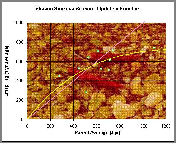
(Picture is from the Canadian Fishing Co.)

A nonlinear least squares fit of the Ricker function above is used on the data and the best Ricker's model for the Skeena sockeye salmon population from 1908-1952 is given by

P_n+1 = R(P_n) = 1.535P_nexp(-0.000783P_n).

Before we analyze this model, we simulate the model using the initial average in 1908 as our starting point and see how well the model traces the data above. Below is a graph of this simulation.

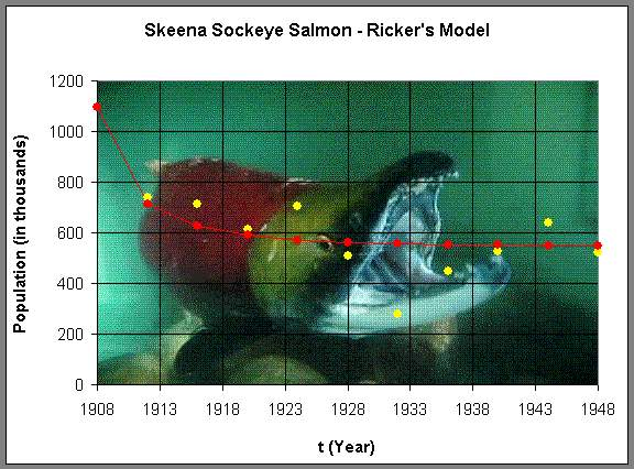
(Picture is from GBarkman Art and Design.)

We see that the Ricker's model has the population leveling off at a stable equilibrium around 550,000, which is relatively consistent with the data. There are a few fluctuations, which is what we would expect from the variations in the environment. However, the model suggests that this is a robust ecological system that maintains a healthy population. Below we will perform a more detailed analysis of this model and use the techniques that we have developed in earlier sections to find equilibria, graph the Ricker's function, and determine the stability of the Ricker's model.

Analysis of the Ricker's Model

As in the logistic model, Ricker's model has two equilibria with one of them being the trivial or zero equilibrium. Let us find the equilibria for this model. As before, the equilibria are found by setting P_e = P_n+1 = P_n, which gives

From this equation, we readily see that P_e = 0 or P_e = ln(a)/b. In lab, we saw that the stability of the equilibria were related to the derivative of the updating function evaluated at the equilibrium. Thus, for Ricker's model, the stability condition for the equilibria is given by

Thus, we need to be able to take the derivative of the updating function. This function is different from previous functions that we have taken the derivative of, in that its the product of two functions that we have been able to differentiate.

Product Rule

Let f(x) and g(x) be differentiable functions. The product rule for finding the derivative of the product of these two functions is given by:

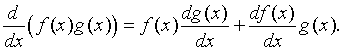
In words, this says that the derivative of the product of two functions is the first function times the derivative of the second function plus the second function times the derivative of the first function.

Example 1: We begin by verifying the product rule with a simple example. Consider f(x) = x⁵. We know that f '(x) = 5x⁴. Let f₁(x) = x² and f₂(x) = x³, then f(x) = f₁(x) f₂(x). From the product rule we have

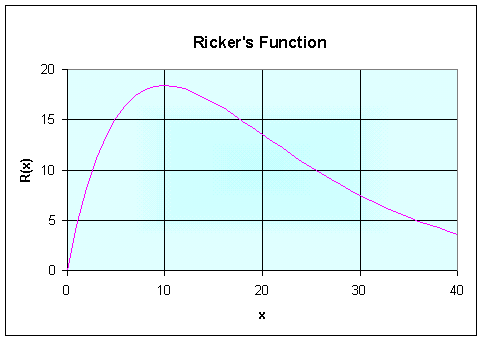
Example 2: Consider the function R(x) = 5x e^-0.1x. Let us sketch a graph of this function, finding all extrema and points of inflection.

Solution: First we note that the only intercept is the origin, (0, 0). Next we use the product rule to differentiate this function.

Since the exponential function is never zero, R '(x) = 0 implies that the only critical point satisfies 1 - 0.1x = 0 or x = 10. Thus, there is a maximum at (10, 50 e^-1) or (10, 18.4).

Next we take the second derivative or the derivative of R '(x). Again we use the product rule to obtain

The point of inflection is found by solving R ''(x) = 0, which is very similar to our equation for the critical point. Its not hard to see that the point of inflection occurs at x = 20. Thus, there is a point of inflection at (20, 100 e^-2) or (20, 13.5).

Simulation of Ricker's Model

Consider Ricker's model given by the equation

where a is a parameter that we will vary to show different behavior. From the discussion above, we have that the equilibria for this equation are

We apply the product rule to R(P) and obtain

Recall that the stability condition for the equilibria is given by

First, we analyze the stability of P_e = 0. However,

which is unstable for a > 1.

Next we consider P_e = 100 ln(a). Substituting into the formula for the derivative gives

Thus, for |R '(100 ln(a))| < 1, we must have a < 7.389.

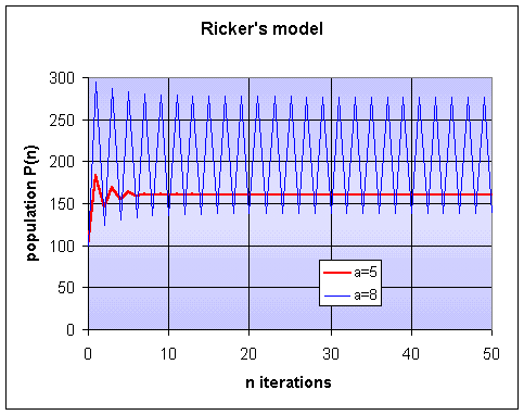
Let us examine simulations for the Ricker's model above with a = 5 and a = 8. The simulations for 50 generations for each of these cases are shown below, where we begin with an initial population P₀ = 100. It is clear that for a = 5 the model tends towards the equilibrium P_e = 161, while the a = 8 case oscillates between the two values of P = 139 and P = 277.

 

As usual, there are several Worked Examples that should help you with the homework problems.

Sockeye Salmon of Skeena River Revisited

From the notes above we have that the best Ricker's model for the Skeena sockeye salmon population from 1908-1952 is

P_n+1 = R(P_n) = 1.535P_nexp(-0.000783P_n).

Let us show the equilibria and stability of the equilibria for this particular case. If we let P_e = P_n+1 = P_n, then

Thus, the two equilibria are P_e = ₀ and _547.3 with the latter equilibrium value close to the value observed in the graph of the simulation above.

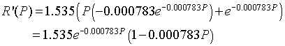
Next we differentiate R(P) and see that

Thus, at _{Pe = 0},

R'(0) = 1.535 > 1,

which shows that the equilibrium at 0 is unstable as expected. However, at P_e = _547.3,

R'(547.3) = 1.535e-0.4285(1 - 0.4285) = 0.571 < 1,

which implies that this equilibrium is stable with solutions monotonically approaching the equilibrium, as we observed in the simulation.

References

[1} Ricker, W.E. 1958. Handbook of computations for biological statistics of fish populations. Fisheries Research Board of Canada.

[2] Shepard, M. P. and Withler, F. C. (1958) Spawning stock size and resultant production for Skeena Sockeye. J. Fisheries Research Board of Canada 15: 1007-1025.

[3] Walters, C.J. 1986. Adaptive management of renewable resources. Macmillan (NY).

[4] Walters, C.J. and Hilborn, R. 1968. Ecological optimization and adaptive management. Annual Rev. of Ecology and Systematics 9, 157-188.