Math 121 - Calculus for Biology I Spring Semester, 2001 Product Rule - Examples
	© 2001, All Rights Reserved, SDSU & Joseph M. Mahaffy San Diego State University -- This page last updated 13-May-00

1. Differentiation of Functions with a Product
2. Application to Graphing
3. Ricker's Growth Model

When a function can only be written as the product of two or more differentiable functions, then the product rule is needed to find the derivative. Several examples are provided to supplement the lecture section and help with the homework problems. The examples include basic differentiation, a graphing example (finding a minimum), and additional studies of the Ricker's model.

Differentiation of Functions with a Product

Example 1: Consider the function given by

Find the derivative of f(x) by using the product rule. Next multiply the terms in f(x), then take the derivative of the resulting polynomial. Show that these give the same functions, verifying the product rule.

Solution: The product rule is carried out by multiplying the first term times the derivative of the second term, plus the second term multiplied by the derivative of the first term.

We should be able to obtain the same result by multiplying the terms in f(x) and then taking the derivative of the resulting polynomial.

Thus, it is easy to see that the two methods do indeed yield the same result.

Example 2: Consider the function given by

Find the derivative of g(x) by using the product rule.

Solution: Again we multiply the first term times the derivative of the second term and add the second term multiplied times the derivative of the first term. Recall that the derivative of the natural logarithm equals the inverse of the argument.

Application to Graphing 

One of the primary applications of the derivative is finding the critical points where minima and maxima occur, which aids in sketching a graph.

Example 3: Consider the function given by

Determine the domain of the function and find any intercepts. Find any critical points, then sketch the graph of f(x) for 0 < x < 2.

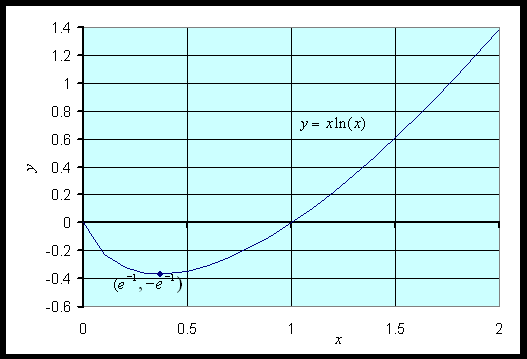
Solution: The domain of the function is x > 0. Thus, there is no y-intercept. However, it can be shown that the limit as x tends to 0 from the right is 0. (You can show this with your calculator, but proof of this result requires more advanced Calculus techniques.) The x-intercept is readily found by solving f(x) = 0, which gives x = 1.

To find the critical points we differentiate f(x) and set it equal to zero, giving

Thus, the critical value of x_c satisfies ln(x_c) = -1 or x_c = e^-1 ~ 0.3679. The function value at the critical point is f(e^-1) = - e^-1 ~ -0.3679. Thus, there is a minimum on the graph at (e^-1, - e^-1). The graph of the function is seen below.

 

Ricker's Growth Model

Example 4: Let P_n be the population of fish in any year n. Consider Ricker's model for population growth given by the equation

where a = 7 and b = 0.02. Sketch a graph of R(P) with the identity function, showing the intercepts, all extrema, and any asymptotes. Find all equilibria of the model and describe the behavior of these equilibria. Let P₀ = 100, and simulate the model for 50 years, graphing the solution.

Solution: First, we see that the only intercept is the origin, (0, 0). Since the negative exponential dominates in the function R(P), there is a horizontal asymptote of P_n+1 = 0. To find the extrema, we differentiate R(P). Applying the product rule we obtain:

This expression is zero only when 1 - 0.02P = 0 or P_c = 50. Thus, there is a critical point for the updating function at

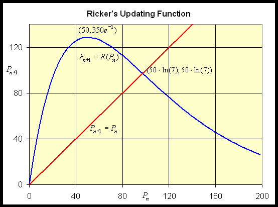
The graph of the updating function along with the identity function is shown below. They intersect at the equilibria, which are calculated later.

To find the equilibria, we substitute P_e for P_n+1 and P_n in the Ricker's model. The resulting equation is given by

One equilibrium is given by P_e = 0, so we can divide out P_e, leaving

This gives the other equilibrium P_e = 50 ln(7) ~ 97.3.

To find the behavior of the solution near each of these, we must substitute the value of the equilibrium into the expression for the derivative. First, we analyze the stability of P_e = 0. We see that,

which is unstable, and the population grows away from the equilibrium P_e = 0.

Next we consider P_e = 50 ln(7). Substituting into the formula for the derivative gives

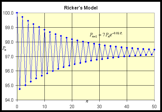
Thus, -1 < R '(50 ln(7)) < 0, so we have a stable equilibrium point with solutions oscillating, but approaching the equilibrium, P_e = 50 ln(7).

The simulation with P₀ = 100 is shown in the graph below. The solution is slowly oscillating toward the equilibrium, as can be seen with 50 iterations.

Example 5: Repeat the previous problem with a = 9.

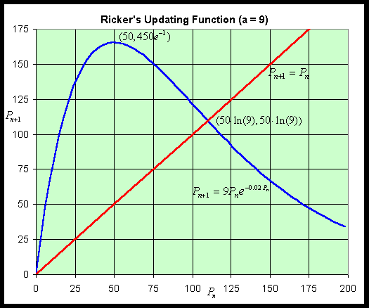
Solution: Many of the computations carry over from the example above. The only intercept is the origin, (0, 0), and there is a horizontal asymptote of P_n+1 = 0. The derivative is only slightly changed as the leading constant is the only variation, so

As in the previous example, the critical point satisfies P_c = 50, which gives a maximum at

The graph of the updating function along with the identity function is shown below with the important points labeled.

The equilibria are found just like the previous example by using P_e for P_n+1 and P_n in the Ricker's model. The resulting equation is given by

The calculations are very similar giving the two equilibria, P_e = 0 and P_e = 50 ln(9) ~ 109.86.

The stability analysis uses the same techniques as before, but the behavior changes at the upper equilibrium. Near P_e = 0, we evaluate the derivative and obtain

which is unstable with the population growing away from this equilibrium.

Near P_e = 50 ln(9), we find that

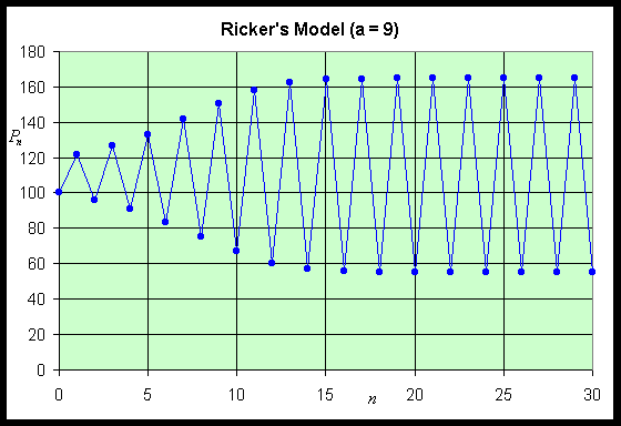
Thus, R '(50 ln(9)) < -1, so we have an unstable equilibrium point with solutions oscillating and moving away from the equilibrium. Below is a simulation with 30 iterations, starting with P₀ = 100. Clearly, the solution oscillates with increasing amplitude. The solution goes to a period 2 behavior, oscillating between 55 and 165.