|
|
Math 121 - Calculus for Biology I |
|
|---|---|---|
|
|
San Diego State University -- This page last updated 03-Apr-01 |
|
Logistic Growth and Nonlinear Dynamical Systems
- Logistic Growth Model
- Yeast Model
- U. S. Census Revisited
- Equilibria
- Worked Examples
- Other Behavior of the Logistic Growth Model
- Reference
Discrete Logistic Growth Model
In an earlier section we studied the Discrete Malthusian growth model, which showed exponential growth. This model is appropriate for early phases of population growth for most animal populations. However, as a population grows, it encounters crowding pressure due to many factors such as toxic build up or space and resource limitation.
In 1913, Carlson [1] studied a growing culture of yeast.
Below is a table of the population for these yeast at one hour intervals. We
would like to develop a mathematical model to describe the growth of this culture.
|
|
|
|
|
|
|
|
|
|
|
|
|
|
|
|
|
|
|
|
|
|
|
|
|
|
|
|
|
|
|
|
|
|
|
|
|
|
|
|
|
|
|
|
|
|
|
|
|
The general discrete dynamical system is given by the
This is an iterative map where the population at the (n + 1)st generation depends on the population at the nth generation. The function f(p) is called the updating function as it produces the next population in the iterative scheme. A graph of the updating function has the (n + 1)st generation on the vertical axis, while the nth generation is on the horizontal axis.
It is clear that the population of yeast in the table above does not satisfy a Malthusian growth, which has a linear updating function and grows exponentially without bound. The next obvious addition to the updating function is the addition of a quadratic term, which should be negative to reflect a decrease in the growth of a population due to crowding effects. This is the Logistic Growth model and can be written:

This equation has the Malthusian growth model seen in the previous section with the additional term -rPn2/M. The parameter M is called the carrying capacity of the population.
The behavior of the Logistic growth model is substantially more complicated than that of the Malthusian growth model. There is no exact solution to this discrete dynamical system. The ecologist Robert May (1974) studied this equation for populations and discovered that it could produce very complicated dynamics. In its simplest form the Logistic growth model can be written:
where the parameter m varies between 0 and 4. For a good description of this model complete with Java applet simulations see the website of B. Fraser.
The graph below shows a plot of pn+1 vs. pn from the
table above. (This is accomplished by plotting the population from one time
against the population from the previous time. For example, the first two points
are (9.6, 18.3) and (18.3, 29.0).) The graph of the data is fit applying Excel's
polynomial fit with trendline, using a quadratic passing through the origin,
and is shown below. The graph of the line pn+1
= pn (the identity map) is also shown, and its importance
for studying discrete dynamical models will be discussed later. This equation
becomes the updating function.
Our discrete logistic growth model for the yeast experiment above is given by
Below is a simulation showing both the data and the model. As we can see, the model does a fairly reasonable job of simulating the data from this fairly simplistic model.
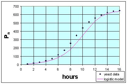
Qualitatively, we see the same initial roughly exponential growth, then both models seem to level off at approximately the same value. This is the carrying capacity of the population. The equation above shows r = 0.56 and r/M = 0.000861, so M = 650.4. This is clearly a little low based on the original table. Furthermore, the model is shifted in time, not rising as soon as the original data.
U. S. Census with Logistic Growth Model
We saw that the Malthusian growth model did not work well for the U. S. census data. Can we apply the logistic growth model to the U. S. census data and get a better fit to the data and avoiding the problems of the time varying nonautonomous model developed at the end of the last section?
We return to the U. S. census data in the previous section. As with the yeast model shown above, we need to find the updating function by plotting Pn+1 versus Pn. So it remains a question of how to best fit an updating function of the quadratic form given by the Logistic growth model through this data. It turns out that if you simply perform the least squares best fit of a quadratic function (without the constant term) through this data (as trendline does in Excel), it gives too much weight to the later years of the model and grossly underestimates the rate of growth r. Based on the assumptions of the Logistic growth model that increasing population should decrease the growth rate, I chose r = 0.351 (matching the initial growth rate between 1790 and 1800), then performed a least squares best fit to the data. This gave the Logistic growth model:
The graph of this updating function with the data is seen below (the line Pn+1 = Pn is usually shown for reference and can be used in a process called cobwebbing that we will not discuss at this time):
The simulation of this discrete Logistic growth model compared to the two models of the previous section and with the data is seen below:
It is clear that the discrete Logistic growth model follows the data better than the Malthusian growth model (even the Malthusian model with r = 0.349), but not as well as the non-autonomous growth model of the previous section. The Logistic growth model shown above predicts the population relatively well up until 1900. However, it even has the wrong concavity after 1930, suggesting a premature leveling off of the population of the U. S. Thus, a time varying growth rate seems the best of these three models. This shows that human populations have a more complicated dynamics than these models can predict with both time-varying and crowding factors. (Sociological and technical factors are especially difficult to incorporate into mathematical models.) Your ecology courses should help explain more details underlying the assumptions in these models, so explain a little better when the models are applicable and why they fail in other predictions.
Later we would like to study the qualitative behavior of discrete dynamical equations in more detail. Consider the general discrete dynamical equation:
The first step in any analysis is finding equilibria, which is simply an algebraic equation (and the area that we are reviewing now). An equilibrium point of a discrete dynamical system is a point where there is no change in the variable from one iteration to the next. Mathematically, this occurs whenever there is a solution to
Graphically, this is when f(P) crosses the line y = P, which is one reason why this line was shown above.
Consider the original discrete Logistic equation listed above with r > 0. The equilibria are found by solving:
Thus, the equilibria for the Logistic growth model are either the trivial solution 0 (no population) or the carrying capacity M.
If we examine the Logistic growth model proposed above for the U. S. census data, then we find the equilibria satisfying:
Thus, Pe = 0 or 2.849*108. Note that this later population is very close to the 2000 census value, while actual projections have the U. S. population rising to over 400 million by the middle of the next century. It is unlikely that human population can continue its current course, but what will be the actual scenario? Mathematical modeling can provide reasonable estimates for short term growth and allows one to predict several different possibilities for longer term depending on the assumptions that are entered into the model.
There are Worked Examples available to help you understand the material.
Other Behavior of the Logistic Growth Model
Below we present an applet that shows simulations of the logistic growth model for various choices of r.
Robert May (1974) demonstrated that the discrete Logistic growth model could display very complicated dynamics.Watch what happens in the applet above as we choose different values of r. For example, try the values r = 0.5, 1.8, 2.3, and 2.65. (Note that the solution of the discrete Logistic equation only gives solutions at the integer values of n, so the connecting lines are only drawn to help visualize the behavior of the system.) The first value of r shows the curve smoothly ascending to carrying capacity of 1000. The second value of r has the population ascend and actually overshoot 1000, then oscillates about 1000, getting closer to the carrying capacity as n increases. In both of these cases, the equilibrium population of 1000 is said to be stable. When r = 2.3, the solution oscillates about 1000, taking on the values of approximately 690 and 1180. This solution is said to have a period of 2. The last case shows the population oscillating almost randomly about 1000. This last situation could have either a very high period of oscillation or actually be chaotic.
Cobwebbing
In the previous section, we introduced a more geometric way to visualize these dynamical systems, cobwebbing. The website of B. Fraser shows this cobwebbing for the logistic growth model in a nice applet. The updating function, f(pn), is graphed with the identity map, pn+1 = pn on a single graph with the vertical axis being pn+1 and the horizontal axis being pn. The idea is that you start at any p0, then go vertically to p1 = f(p0). Next you go horizontally to the identity map to locate p1 on the horizontal axis. From there you find p2 by going vertically to p2 = f(p1). This process is repeated to generate the cobweb of points by this discrete dynamical system. The sequence of points on the horizontal axis form the solution set generated by the discrete dynamical system. The graphical representation allows you make some projections of the behavior of the system. Below is a diagram showing several steps in the cobwebbing scheme for the quadratic map
[1] T. Carlson Über Geschwindigkeit und Grösse der Hefevermehrung in Würze. Biochem. Z. 57: 313-334, 1913.