![]()
Math 121 - Calculus for Biology I
Spring Semester, 2004
Limits, Continuity, and the Derivative
San Diego State University -- This page last updated 30-Dec-03
|
|
Math 121 - Calculus for Biology I |
|
|---|---|---|
|
|
San Diego State University -- This page last updated 30-Dec-03 |
|
This is a theoretical section that studies the concepts of limits, continuity, and the derivative. This section provides the definition of the derivative given near the end of this section.
This section contains a sketch of the formal mathematics that is required to fully develop the concept of the derivative. A complete understanding is beyond the scope of this course, but a few of the ideas are sufficiently important that some discussion is warranted. In the previous sections we have discussed how the derivative is related to the slope of the tangent line for a curve at a point. This was viewed geometrically by considering a sequence of secant lines that approached the tangent line at a point or algebraically by examining what happened to the slope computed at a point as you took points closer and closer together on the curve. (Another perspective on this subject can be viewed in the University of British Columbia notes, which have had more time to be developed.)
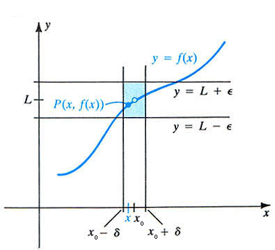
Both the geometric and the algebraic ideas mentioned above need the concept of a limit. From a conceptual point of view, the limit of a function f(x) at some point x0 simply means that if your value of x is very close to the value x0, then the function f(x) stays very close to some particular value.
Definition: The limit of a function f(x) at some point x0 exists and is equal to L if and only if every "small" interval about the limit L, say the interval (L - e, L + e), means you can find a "small" interval about x0, say the interval (x0 - d, x0 + d), which has all values of f(x) existing in the former "small" interval about the limit L, except possibly at x0 itself.
This is a difficult concept to fully appreciate. However, you should be able to grasp the idea through several examples.
Examples:
1. Consider f(x) = x2 - x - 6. Find the limit as x approaches 1. It is not hard to see from either the graph or from the way you have always evaluated this quadratic function that as x approaches 1, f(x) approaches -6, since f(1) = -6.
Fact: Any polynomial, p(x), has as its limit at some x0, the value of p(x0).
2. Consider the rational function r(x) = (x2 - x - 6)/(x - 3). Find the limit as x approaches 1. If x is not 3, then this rational function reduces to r(x) = x + 2. So as x approaches 1, this function simply goes to 3.
Fact: Any rational function, r(x) = p(x)/q(x), where p(x) and q(x) are polynomials with q(x0) not zero, then the limit exists with the limit being r(x0).
3. Consider the rational function in Example 2. Now f ind the limit as x approaches 3. Though r(x) is not defined at x0 = 3, we can see that arbitrarily "close" to 3, r(x) = x + 2. So as x approaches 3, this function simply goes to 5. Its limit exists though the function is not defined at x0 = 3.
4. Consider the rational function f(x) = 1/x2. Find the limit as x approaches 0, if it exists. From our statement above on rational functions, this function has a limit for any value of x0 where the denominator is not zero. However, at x0 = 0, this function is undefined. Thus, the graph has a vertical asymptote at x0 = 0. This means that no limit exists for f(x) at x0 = 0.
Fact: Whenever you have a vertical asymptote at some x0, then the limit fails to exist at that point.
5. Consider the rational function r(x) = (x2 - x - 2)/(x - 3). Find the limit as x approaches 3, if it exists. From our statement above on rational functions, this function has a limit for any value of x0 where the denominator is not zero. However, at x0 = 3, this function is undefined; and furthermore, the function is not approaching zero in the numerator near x0 = 3. Thus, the graph would show a vertical asymptote at x0 = 3. This means that no limit exists for r(x) at x0 = 3.
6. The Heaviside function is often used to specify when something is "on" or "off." The Heaviside function is defined as
This function clearly has the limit of 0 for any x < 0, and it has the limit of 1 for any x > 0. Even though this function is defined to be 1 at x = 0, it does not have a limit at x0 = 0. This is because if you take some "small" interval about the proposed limit of 1, say e = 0.1, then all values of x near 0 must have H(x) between 0.9 and 1.1. But I can take any "small" negative x and H(x) = 0, which is not in the desired given interval. Thus, no limit exists for H(x).
Perspective: Whenever a function is defined differently on different intervals in a manner similar to the Heaviside function above, you need to check the places where the function changes in definition to see if the function has a limit at these x values where the function changes. (It might also have asymptotes at other points where again you would check.)
7. Consider the fractional power function f(x) = x1/2. Find the limit as x approaches 0, if it exists. This function is not defined for x < 0, so it cannot have a limit at x = 0, though it is said to have a right-handed limit.
Summary of Limits: Most of the functions that you regularly examine have limits. Usually, the problems arise at points x0 when there is a vertical asymptote, the function is defined differently on different intervals, or special cases like the square root function.
Closely connected to the concept of a limit is that of continuity. Intuititvely, the idea of a continuous function is what you would expect. If you can draw the function without lifting your pencil, then the function is continuous. Most practical examples use functions that are continuous or at most have a few points of discontinuity.
Definition: A function f(x) is continuous at a point x0 if the limit exists at x0 and is equal to f(x0).
The examples above should also help you appreciate this concept. In all of the cases except Example 3, the existence of a limit also corresponds to points of continuity. Example 3 is not continuous at x0 = 3 though a limit exists here, as the function is not defined at 3. Examples 3 and 5 are discontinuous only at x0 = 3, while Examples 4, 6 and 7 are discontinuous only at x0 = 0. At all other points in the domains of these examples are continuous.
Example Comparing Limits and Continuity
An example is provided to show the differences between limits and continuity. Below is a graph of a function, f(x), that is defined on the interval [-2, 2], except at x = 0, where there is a vertical asymptote.
It is clear that the difficulties with this function occur at integer values. At x = -1, the function has the value f(-1) = 1, but it is clear that the function is not continuous nor does a limit exist at this point. At x = 0, the function is not defined (not continuous nor has any limits) as there is a vertical asymptote. At x = 1, the function has the value f(1) = 4. The function is not continuous at x = 1, but the limit does exist with
![]()
At x = 2, the function is continuous with f(2) = 3, which also means that the limit exists. At all non-integer values of x the function is continuous (hence its limit exists).
The primary reason for the discussion above is to give you the proper definition of the derivative. In the previous sections, we noted that the derivative at a point on a curve is the slope of the tangent line at that point. This motivation is what underlies the definition given below.
Definition: The derivative of a function f(x) at a point x0 is denoted by f '(x0) and satisfies
provided this limit exists.
Examples:
1. Let us use this definition to find the derivative of f(x) = x2.
2. We repeat this computation to find the derivative of f(x) = 1/(x + 2) (for x not equal to -2).
Clearly, we do not want to use this formula every time we need to compute a derivative. The next section gives much easier formulae for finding derivatives. (Another very easy way to find derivatives is using the Maple diff command, which we will also discuss.)