Math 121 - Calculus for Biology I Spring Semester, 2001 Quotient Rule
	© 2001, All Rights Reserved, SDSU & Joseph M. Mahaffy San Diego State University -- This page last updated 11-May-01

1. Mitotic Model
2. Quotient Rule
3. Hassell's Model
4. Worked Examples
5. Chalone Model Analysis
6. References

The last section developed the product rule as another differentiation technique. There were applications of the product rule to Ricker's model for population growth and to graphing problems. In this section, we examine a mitotic model and an alternative model developed by Hassell for population growth with each of these models having a quotient rather than a product. In earlier sections, we studied graphing of rational functions, but had no techniques for finding critical points. The ability to find the derivatives of rational functions allows locating minima and maxima of these functions.

Mitotic Model

Multicellular organisms begin with exponentially growing cell populations (Malthusian growth), but soon must regulate this cell growth to develop particular patterns and shapes and differentiate their cells into organs with specific functions. The adult organism maintains a fairly constant number of cells, which means that cells must recognize whether or not there is a need to divide, a process known as mitosis. Cancer is often the breakdown of this control, with cells dividing when they normally would not. One significant question that has yet to be adequately answered is how a cell, such as a skin cell, recognizes its neighboring environment of other cells and knows whether or not it should divide. (A skin cell obviously needs to undergo mitosis when either wear or damage of the skin requires replacement cells.)

The regulation of mitosis is a very important biological process that is currently being studied extensively. This research tries to understand how cells determine when they should undergo mitosis. One controversial biochemical theory developed in the late 1960s was that cells communicated with neighboring cells by tissue-specific inhibitors known as chalones [1]. The chalones are released by cells and diffuse in the environment to affect the cells nearby. If there are sufficient quantities of these chalones, then cells are inhibited from undergoing mitosis.

One of the proposed mechanisms is that chalones bind specifically to certain proteins involved in mitosis. The chalones inactivate the mitotic proteins, leaving the cell in a quiescent state. This inhibition process of effector molecules binding to a protein is often modeled using a Hill function, which has a special rational form. Let P_n represent a certain population of cells, then using a Hill function to simulate the effect of chalones, we propose the following discrete dynamical model for mitosis:

where a = 2 represents one cell dividing into 2 cells and b and c are parameters that could be fit to data. This discrete dynamical model's updating function is a quotient.

Analysis of the behavior of the chalone model uses the standard techniques that we have developed earlier in this course. Notice that when the population P_n is very low, then the denominator of the model is insignificant, so by ignoring it, we see the standard Malthusian growth model. However, large populations increase the denominator resulting in a decline in production of the generation of cells. We would like to determine equilibria of this model and find the stability of those equilibria. From before, the stability of the model's equilibria depends on the value of the derivative of f(P) at the equilibria, which means we must be able to differentiate the quotient given in f(P).

Quotient Rule

Let f(x) and g(x) be two differentiable functions. The quotient rule for finding the derivative of the quotient of these two functions is given by:

where f '(x) and g'(x) are the derivatives of the respective functions. In words, the quotient rule says that the derivative of the quotient is "the bottom times the derivative of the top minus the top times the derivative of the bottom all over the bottom squared."

Example: Suppose we want to study the function

We can apply the quotient rule to this function to find its derivative. We obtain

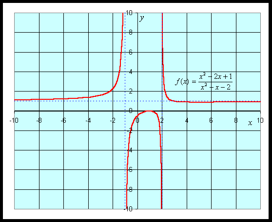
For graphing this function, we would like to find intercepts, asymptotes, and extrema. The y-intercept is given by y = f(0) = -1/2. The x-intercept is found by solving f(x) = 0. This is solved by setting the numerator equal to zero, but

which gives the x-intercept as x = 1.

The vertical asymptotes are found finding when the denominator is zero, so

This gives the vertical asymptotes x = -1 and x = 2. The horizontal asymptote is found by looking at f(x) for large values of x. The largest exponents in the numerator are both 2, so for large x, f(x) behaves like x²/ x² = 1, which gives the horizontal asymptote y = 1.

The critical points are found by setting the derivative equal to zero, which again requires setting the numerator equal to zero. Thus,

Thus, the critical points are x_c = 1 and x_c = 5. Evaluating the function f(x) at these critical points, and we find a local maximum at (1, 0) and a local minimum at (5, 8/9). A graph of this function is seen below.

 

Hassell's Model

Other alternatives to the Logistic growth model and Ricker's model have been developed. One that is frequently applied to insect populations is Hassell's model, which is written in the form of a quotient. One form of this model is given by the following:

In the next section on the chain rule, we will study the more general Hassell's model. The numerator of H(P_n) is the Malthusian growth model, so that at low population densities, the population grows exponentially. (Recall that this requires a > 1.) As the population increases, the denominator increases, which slows the rate of growth. As before, we would like to study the behavior of this discrete dynamical model. In the next section, we will apply this model to actual data from insect populations.

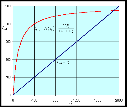
First, we would like to graph the updating function, H(P_n), for P_n > 0 to show the growth rate behavior described above. It is clear that the only intercept is (0, 0). The vertical asymptote for this function is outside the domain, but there is a horizontal asymptote at H = a/b. Biologically, this implies that there is a maximum number in the next generation, no matter how large the population starts (which is reasonable considering limited resources). Thus, the population (after the initial population) must always remain below P_n = a/b. If we differentiate H(P), we use the quotient rule to obtain

Notice that H '(P) > 0, so H(P) is always increasing. Thus, the graph starts at H(0) = 0, then increases and approaches the asymptote H = a/b. Below we let a = 20 and b = 0.01 to produce the following graph shown with the identity map.

Following the usual techniques for studying discrete dynamical models, we next find the equilibria of this model by letting P_e = P_n = P_n+1. Thus, we solve

Simplifying this last expression gives

As is common for population models, we have the trivial equilibrium and then a larger value, which corresponds to the carrying capacity of this population.

We expect the behavior of the model near the zero equilibrium to grow exponentially away from 0. We can see that

by the assumption on a. Thus, our properties on the stability of discrete dynamical models give the zero equilibrium as being unstable and having solutions grow monotonically away from this equilibrium.

At P_e = (a - 1)/b, we can easily compute the derivative obtaining

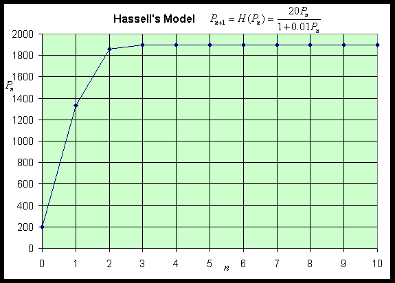
Thus, our properties on the stability of discrete dynamical models give P_e = (a - 1)/b as being stable with all solutions monotonically approaching this equilibrium. Below we show a simulation of 10 iterations for our specific example above with P₀ = 200. This simulation shows the predicted behavior.

For more examples, see the Worked Examples section.

Chalone Model Analysis

We return to the model for mitosis. The standard analysis of the discrete dynamical models is to find equilibria, then examine the derivative of the updating function near at the equilibria. We can write the chalone model above in the following form:

If we substitute P_e = P_n = P_n+1 into the chalone model, then we have

The equation above shows that the equilibria are P_e = 0 or P_e = 1/b.

The next step is to differentiate the updating function. The quotient rule gives

From the expression above, we see that f '(0) = 2, while f '(1/b) = (2 - c)/2. Thus, we see that the solution grows monotonically away from the unstable equilibrium P_e = 0, while the stability and behavior of the equilibrium P_e = 1/b depends on the value of c. A specific example is in the Worked Examples section.

References

[1] W. S. Bullough and E. B. Laurence (1968) Chalones and cancer, Nature 220, 134-135.