|
|
Math 121 - Calculus for Biology I |
|
|---|---|---|
|
|
San Diego State University -- This page last updated 22-Aug-03 |
|
|
|
Math 121 - Calculus for Biology I |
|
|---|---|---|
|
|
San Diego State University -- This page last updated 22-Aug-03 |
|
Link
to Assignment and Quiz Page
This course is the first semester of the Calculus for Biology sequence at SDSU. The science of Biology is rapidly expanding with an increased need for more quantitative analysis of the data. Thus, mathematics and computers are becoming more important to researchers in Biology. My emphasis for this course will be mathematical modeling of biological systems. (My specialty in research is mathematical biology, so you may find my approach quite different from other math courses that you've seen in the past.) The lecture notes are designed to show how Calculus naturally arises in biological examples from classical and current research. Most sections will begin with a biological model that motivates some aspect of learning Calculus. The example is followed by the mathematical theory required to analyze the biological problem and other related problems. Most sections will include hypertext links to worked examples that will illustrate the types of problems you will encounter in the homework sets. Often additional biological examples are provided after the theoretical section to demonstrate the wide range of applicability of the mathematical techniques.
Biological examples are inherently complex, which complicates the understanding of how mathematical modeling relates to the biological problems. Typical courses in the past use grossly simplified examples, which have resulted in students feeling that Calculus is irrelevant to their study of Biology. My web-based course attempts to use more convincing examples and has a significant portion devoted to computer labs, where technology can aid with the more complicated models. The course is taught with two lectures per week using these web-based notes and one lab period each week where we meet in the computer lab to work on related problems. The computer labs will use a mix of computer techniques, which are detailed in the introduction to the lab section. Be sure to review the introductions to the other sections on this website to familiarize yourself with my approach to this course.
Biology is one of the most rapidly expanding and diverse areas in the sciences. The problems encountered in Biology are frequently complex and often not totally understood. Mathematical models provide a means to better understand the processes and unravel some of the complexities. This gives a natural synergistic relationship between the two fields as research expands in the future. The mathematical tools provide ways of developing a better qualitative and quantitative understanding of some biological problems, while the biological problems often stretch the techniques that mathematicians must use to find solutions.
A mathematical model is a representation of a real system. The essence of a good mathematical model is that it is simple in design and exhibits the basic properties of the real system that we are attempting to understand. The model should be testable against empirical data. The comparisons of the model to the real system should ideally lead to improved mathematical models. The model may suggest improved experiments to highlight a particular aspect of the problem, which in turn may improve the collection of data. Thus, modeling itself is an evolutionary process, which continues toward learning more about certain processes rather than finding an absolute reality. This use of mathematics is quite different from K-12 training in mathematics, where mathematics is treated as an absolute with exact answers.
Example 1: Diabetes mellitus
An ongoing example of the modeling process is provided by diabetes mellitus. This is a metabolic disease which is characterized by too much sugar in the blood and urine. In a normal subject the b-cells in the pancreas release insulin in response to rises in levels of glucose in the blood, which results in the storage of this source of energy as glycogen in the liver. (The figure behind the graph above shows the islets of Langerhans, which contain the b-cells.) One form of the disease (Type I) has its onset in childhood and is caused by a failure of the b-cells to release insulin in response to blood glucose levels. It appears that this form of diabetes is caused by antibodies being formed that react with islet cells, then the subsequent autoimmune response selectively destroys the b-cells. Thus, insulin can no longer be produced. Another form (Type II) appears in adults (and increasingly among obese children). Some cases of Type II diabetes also appear to be an autoimmune disease where the immune system mounts an attack on the b-cells, decreasing their ability to produce insulin, while other Type II diabetes cases may simply result from excessive body weight that overtaxes the ability of the b-cells to produce sufficient insulin. In either case the body loses its ability to regulate blood sugar, which can be potentially very dangerous.
One simple test for detection of diabetes is the Glucose Tolerance Test (GTT). For this test, a subject fasts for 12 hours, then is given a large quantity of glucose. For the next few hours, blood samples are drawn and blood glucose levels are measured. The graphs above show two subjects given this GTT. By fitting the data to a simple model by Ackerman et al. [1], the information from the model can indicate which subjects have diabetes. Both the biological test and the mathematical model are overly simplistic, so improved models and biological testing routines have been developed and continue to be developed.
Diabetes is treated by administration of insulin and regulation of diet by the patients. Biological research has improved our understanding of this disease, which has resulted in improved mathematical models for glucose metabolism. The mathematical models in turn are used to suggest better treatments, such as improved scheduling of insulin injections, which improve the quality of life of the patients suffering from this disease.(A complex model for simulation of insulin and dietary adjustment is available on the web.) Due to both new clinical (or experimental) studies and improved mathematical models, future treatments will certainly evolve to better regulate this metabolic problem in patients with diabetes. There are many websites available about diabetes. Some examples include ones on diagnosing diabetes, gestational diabetes, glucose blood testing, or homeostasis. There are other mathematical models that have been developed to study the firing (hence release of insulin) by the b-cells. (For example, Arthur Sherman at NIH has a number of models and links to models of b-cells.)
Example 2: ATP Synthase
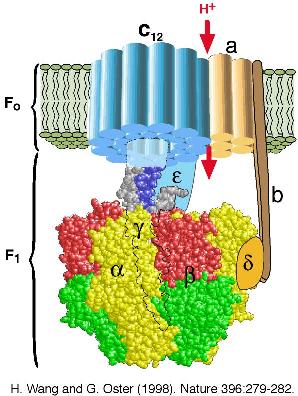
One of the most important molecules in all living organisms is ATP synthase. Cells store chemical energy in two forms: as transmembrane electrochemical gradients and in chemical bonds, particularly the gamma phosphate bond in adenosine triphosphate (ATP). In mitochondria, bacteria, and chloroplasts, the free energy stored in transmembrane electrochemical gradients is used to synthesize ATP from ADP and phosphate via the membrane-bound enzyme ATP synthase. ATP synthase can also reverse itself and hydrolyze ATP to pump ions against an electrochemical gradient. This molecule has been so optimized by evolution that there are few variations in its structure over the entire range of living organisms. Until recently, few details about the structure of this molecule and how it produced ATP were known. The standard texts still talk about how the forming and breaking of the high energy gamma phosphate bond as if it were a single event. Yet the incredibly high efficiency of this molecule (over 90%) could not be explained by physical laws of thermodynamics associated with the cleaving (or forming) of this phosphate from ATP.
A collaboration of many scientist from many fields, including some applied mathematicians, were required to learn the details of how this important molecular reaction occurs. Complicated molecular biology, x-ray crystallography, physics, and mathematical modeling combined to show how phosphate bond was formed in a series of 15 to 20 smaller steps to produce ATP in this highly efficient process. (A Nobel prize in 1997 for Chemistry was awarded to Paul D. Boyer, John E. Walker, and Jens C. Skou for some of the work.) Fundamentally, the scientific discovery followed the diagram given above, where constant exchanges were needed between experimentalists and theoreticians to test that they were converging on the answer of the reality of a remarkable molecule that powers every living cell. For more on the modeling efforts on this important molecule, you might want to check the websites of George Oster and Hongyun Wang.
This course will begin with some linear models. You should check my webpage for more on this material.
References
[1] E. Ackerman, L. Gatewood, J. Rosevear, and G. Molnar, Blood glucose regulation and diabetes, Chapter 4 in Concepts and Models of Biomathematics, F. Heinmets, ed., Marcel Dekker, 1969, 131-156.
[2] E. Krimmel and P. Krimmel, The low blood sugar handbook, Franklin Publishers, 1992, 67-69.