Math 121 - Calculus for Biology I Spring Semester, 2001 Chain Rule
	© 2001, All Rights Reserved, SDSU & Joseph M. Mahaffy San Diego State University -- This page last updated 12-May-01

1. Study of a Beetle Population
2. Chain Rule
3. Analysis of Hassell's Model
4. Worked Examples
5. References

The differentiation in Hassell's model required an additional property of differentiation to complete the computation. Often we encounter composite functions where a function can be written as the composition of two functions. Below we will see that this requires a special rule for differentiation, the chain rule.

Study of a Beetle Population

In the previous section, we examined a special case of Hassell's model for studying the dynamics of insect populations. The more general model, which is applied to insect populations, has the form:

 

where a, b, and c are parameters that are chosen to match the data for a population study of some insect. This is a quotient of two functions with the denominator being a composite function, including a linear function, 1 + bP_n, which is raised to the c power. The denominator is an example of a function that requires the chain rule.

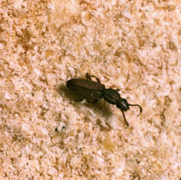
In 1946, A. C. Crombie [1] studied several beetle populations to try to better understand their dynamics under the strict control of a constant amount of food regularly supplied. He maintained the amount of food at 10 grams of cracked wheat added weekly, then regularly took census of the beetle populations. These experimental conditions match the assumptions used by the Logistic growth model. One study was on Oryzaephilus surinamensis, the saw-tooth grain beetle. Below is a table of his data (with some minor modifications to fill in times of uncollected data and an initial one week shift).

By plotting the data of P_n+1 vs. P_n, we can attempt to fit an updating function to the data, then use this updating function to study the population dynamics with an appropriate discrete dynamical model. In this section, we want to study Hassell's model and compare it to the Logistic growth model that we have studied before. Below is a graph showing the best fit to Crombie's data for Oryzaephilus surinamensis for both Hassell's model and the Logistic growth model. (The best fit for Hassell's model was found using the fminsearch routine in MatLab, while the Logistic growth model used Trendline in Excel.)

 

With the 3 parameters to fit the curve to the data, Hassell's updating function is capable of fitting the data better than the quadratic function of the Logistic growth model. It also has the added advantage that it never becomes negative, which was a property that we noted was an improvement in Ricker's model. The best model from Hassell's formula is given by:

 

while the best Logistic growth model satisfies

 

We would like to see how well each of these models simulates the data. With the updating functions, we can readily simulate the discrete dynamical models. Below shows the simulations of the models with the data (assuming the models agree with the data at week 0).

We can readily see that Hassell's model does appear to simulate the data better, especially having the early rapid rise in the population. All seem to tend toward a similar carrying capacity. For more details on the behavior of these models, we would like to perform our standard analysis of the discrete models, locating equilibria and using the derivative to test the local behavior of these models. Finding the derivative of Hassell's model requires the use of the chain rule. 

Chain Rule

Consider the composite function f(g(x)). Suppose that both f(x) and g(x) are differentiable functions. The chain rule for differentiation of this composite function is given by

Example 1: Consider the function h(x) = (x² + 2x - 5)⁵. Find h'(x).

Solution: This can be considered a composite of the function f(u) = u⁵ and the function g(x) = x² + 2x - 5. It is easy to find the derivatives of both f and g. We have f '(u) = 5u⁴ u^' and g'(x) = 2x + 2. From the formula above, we see that

Example 2: Consider the function h(x) = exp(2-x²). Find h'(x).

Solution: This can be considered a composite of the function f(u) = e^u and the function g(x) = 2 - x². The derivatives of f and g are f '(u) = e^u u^' and g'(x) = -2x. From the formula above, we see that

See the Worked Examples section for more examples.

Analysis of Hassell's Model

We return to the general Hassell's model to obtain the equilibria and determine stability conditions for the equilibria. Following the usual techniques for studying discrete dynamical models, the equilibria of Hassell's model are found by letting P_e = P_n = P_n+1. Thus, we solve

This is equivalent to

One of the equilibria is P_e = 0, while the other solves (1 + bP_e)^c = a. This latter equation is easily solved by taking the c^th root of each side, then completing the algebra, so

To determine the stability of the equilibria, we differentiate the function H(P). This requires the quotient rule, which in turn requires differentiating the denominator, which is a composite function. Below we use the chain rule to differentiate the term in the denominator.

Now applying the quotient rule, we find that

This formula can be used to show that H '(0) = a, but since a > 1 for a positive equilibrium to exist, this condition implies that the zero (or trivial) equilibrium in unstable with solutions monotonically growing away from this equilibrium. At the other equilibrium, we can evaluate H '(P_e) and obtain

This calculation shows that the stability of the carrying capacity equilibrium is very dependent on both a and c, but not b. Below we show a series of simulations for Hassell's model with a = 20 and b = 0.01, while c varies. The simulations are for c = 1, 2, 3, and 4. The first three cases are stable, while when c = 4, the model is unstable. We see that for c = 1 the model monotonically approaches its equilibrium at 1900. For c = 2, 3, the solution first oscillates before going to the equilibrium points 347 and 171, respectively. When c = 4, the solution oscillates between 51 and 196.

References:

[1] A. C. Crombie (1946) On competition between different species of graminivorous insects, Proc. R. Soc. (B), 132, 362-395.