1. Annual Temperature Cycles
2. Trigonometric Functions
3. Radian Measure
4. Sine and Cosine
5. Properties and Identities for Sine and Cosine
6. Period, Amplitude, Phase, and Vertical Shift
7. Examples 
8. Worked Examples
9. Return to the Annual Temperature Variation
10. Degree and Radian Conversions
11. References

Many phenomena in biology appear in cycles. Often these cycles are driven by the natural physical cycles that result from the daily cycle of light or the annual cycle of the seasons. Oscillations are most easily studied using trigonometric functions. This section begins with a discussion of annual temperature variations, then we review some trigonometric functions.Many phenomena in biology appear in cycles. Often these cycles are driven by the natural physical cycles that result from the daily cycle of light or the annual cycle of the seasons. Oscillations are most easily studied using trigonometric functions. This section begins with a discussion of annual temperature variations, then we review some trigonometric functions. The emphasis for this section is modeling oscillatory behavior with the sine and cosine functions.

Annual Temperature Cycles

Often the weather report states what the average expected temperature of a given day is. These averages are derived from long term collection of data on weather for a particular location. Clearly, there is a relatively wide variation from these averages, but they provide approximations to the expected weather for a particular time of year. The long term averages also provide a baseline to help researchers determine the predicts effects of global warming over the background noise of annual variation. Obviously, there are seasonal differences in the average daily temperature with higher averages in the summer and lower averages in the winter. Below we provide a table of showing the monthly average high and low temperatures for San Diego and Chicago.

What mathematical tools can help predict the annual temperature cycles? Polynomials and exponentials do not exhibit the periodic behavior that we see for these average monthly temperatures, so these functions are not appropriate for modeling this system. The most natural candidates for studying monthly temperatures are the trigonometric functions. Below are graphs of the average monthly temperatures for San Diego and Chicago, which are computed from the table by averaging the average high and low temperatures.

The two graphs above have some similarities and clear differences. They both show the same seasonal period as expected; however, the seasonal variation or amplitude of oscillation for Chicago is much greater than San Diego. Also, the overall average temperature for San Diego, being further south and near the ocean, is greater than the average for Chicago. The overlying models in the graph above use cosine functions. The fit using the cosine function provides a reasonable approximation though clearly there are errors due to other complicating factors in weather prediction. Before providing more details of the models for these temperature cycles, we review some basic facts about trigonometric functions.

Trigonometric Functions

The trigonometric functions are often called circular functions, which emphasizes their periodic nature and shows their connection to a circle. Let (x, y) be a point on a circle of radius r centered at the origin. Define the angle q between the ray connecting the point to the origin and the x-axis. (See the diagram below.) 

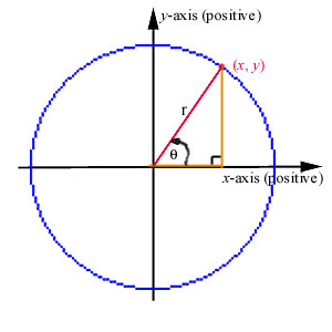
The six basic trigonometric functions are defined in terms of x, y, and r (including the sign of x and y) shown in the diagram above by the following:

We will concentrate almost exclusively on the first two of these trigonometric functions, sine and cosine.

Radian Measure

Before discussing the nature of the trigonometric functions in more detail, we need to discuss radian measure of the angle. If you have had trigonometry before, you probably used degrees to measure an angle. However, they are not the appropriate unit to use in Calculus. The easiest way to consider radian measure is to examine the unit circle (which is simply the circle in the diagram above with a radius of 1). From earlier courses, you may recall that the circumference of a circle is 2pr, so the distance around the perimeter of the unit circle is 2p. The radian measure of the angle q in the diagram above is simply the distance along the circumference of the unit circle. Thus, a 45^o angle is 1/8 of the distance around the unit circle or p/4 radians. Similarly, 90^o and 180^o angles convert to p/2 and p radians, respectively. Below are formulae for converting from degrees to radians or radians to degrees:

A javascript is provided for easy conversions of degrees to radians or radians to degrees through a hyperlink.

Sine and Cosine

From the formulae for sine (sin) and cosine (cos) above, we see that if you take a unit circle, then the cosine function gives the x value of the angle (measured in radians), while the sine function gives the y value of the angle. The tangent function (tan) gives the slope of the line (y/x). Below is a graph of the sine and cosine functions for the angles from -2p to 2p, i.e., the graph shows sin(x) and cos(x) for -2p < x < 2p. (Note that the x here is the angular measurement, which is the q argument above and not the x, which measures the adjacent side of the triangle.)

There are several things to notice about these graphs. First, you notice the 2p periodicity. In other words, the functions repeat the same pattern every 2p radians. This is clear from the circle above because every time you go 2p radians around the circle, you return to the same point. The second point is that both the sine and cosine functions are bounded between -1 and 1. The sine function has its maximum value at p/2 with sin(p/2) = 1 and its minimum value at 3p/2 with sin(3p/2) = -1. Because of the periodicity, these extrema reoccur every integer multiple of 2p.

Below is an applet to help you link the picture of the circle above and the trigonometric functions, sine and cosine, graphed above, using the dynamics of an applet. Click on the applet to place the point. The table below the applet gives the angle in degrees and radians and values of the sine and cosine functions at the angle chosen.

source code for trig6a.class

Below is a table of some important values of the trig functions to remember.

x	sin(x)	cos(x)
0	0	1
p/6	1/2
p/4
p/3		1/2
p/2	1	0
p	0	-1
3p/2	-1	0
2p	0	1

Properties and Identities for Sine and Cosine

There are a number of properties that are significant for sine and cosine.

Properties of Cosine

1. Periodic with period 2p
2. Cosine is an even function
3. Cosine is bounded by -1 and 1
4. Maximum at x = 0 with cos(0) = 1
5. By periodicity, other maxima at x_n = 2np with cos(2np) = 1 (n any integer)
6. Minimum at x = p with cos(p) = -1
7. By periodicity, other minima at x_n = (2n+1)p with cos((2n+1)p) = -1 (n any integer)
8. Zeroes of cosine separated by p with cos( x_n) = 0 when x_n = p/2 + np (n any integer)

Properties of Sine

1. Periodic with period 2p
2. Sine is an odd function
3. Sine is bounded by -1 and 1
4. Maximum at x = p/2 with sin(p/2) = 1
5. By periodicity, other maxima at x_n = p/2 + 2np with sin(x_n) = 1 (n any integer)
6. Minimum at x = 3p/2 with sin(3p/2) = -1
7. By periodicity, other minima at x_n = 3p/2 + 2np with sin((x_n) = -1 (n any integer)
8. Zeroes of sine separated by p with sin( x_n) = 0 when x_n = np (n any integer)

When studying trigonometry, there are many special trigonometric identities that are frequently learned. We are going to highlight a very few that are particularly useful.

Some Identities for Sine and Cosine

1. cos²(x) + sin²(x) = 1 for all values of x
2. Adding and subtracting angles for cosine
   cos(x + y) = cos(x)cos(y) - sin(x)sin(y)
   cos(x - y) = cos(x)cos(y) + sin(x)sin(y)
3. Adding and subtracting angles for sine
   sin(x + y) = sin(x)cos(y) + cos(x)sin(y)
   sin(x - y) = sin(x)cos(y) - cos(x)sin(y)

The first of these identities is readily verified using Pythagorean's Theorem and the definitions of sine and cosine. The second two identities are not as easily shown, and we will omit their proofs here {Proofs use basic definitions of the sine and cosine functions - last visited 8/11}. The second two identities are useful in showing that from a modeling perspective, the sine and cosine functions are often interchangeable.

Example: Use the trigonometric properties and identities to show that

Solution: From the additive formula for sine functions

sin(x + p/2) = sin(x)cos(p/2) + cos(x)sin(p/2)

By our properties above, we know cos(p/2) = 0 and sin(p/2) = 1, so

sin(x + p/2) = cos(x)

This relationship says that the cosine function is exactly the same as the sine function, but shifted out of phase by -p/2 (or the sine curve shifted
to the left by p/2).

Using the subtractive identity formula for cosine functions

cos(x - p/2) = cos(x)cos(p/2) + sin(x)sin(p/2)

Again cos(p/2) = 0 and sin(p/2) = 1, so

cos(x - p/2) = sin(x)

This relationship says that the sine function is exactly the same as the cosine function, but shifted out of phase by p/2 (or the sine curve shifted
to the right by p/2).

Period, Amplitude, Phase and Vertical Shift

The sine and cosine functions above have a period of 2p and an amplitude of one, so how can we adjust these functions to fit other periodic data, such as the temperature data for Chicago and San Diego given in the introduction to this section? hen data follows a simple oscillatory behavior, then a general modeling form using the cosine function is

• The model parameter A is the vertical shift, which is associated with the average height of the model
• The model parameter B gives the amplitude, which measures the distance from the average, A, to the maximum (or minimum) of the model
  

The parameter w is the frequency of the models.

Frequency and Period

• The model parameter w is the frequency, which gives the number of periods of the model that occur as x varies over 2p radians
• The period is given by

T = 2p/w

It is the periodic nature of the models for which these functions have been chosen. The last parameter, f, is the phase shift.

Phase Shift

• The model parameter f is the phase shift, which shifts our models to the left or right, thus, gives a horizontal shift
• If the period is denoted T = 2p/w, then the principle phase shift satisfies 0 < f < T
• By periodicity of the model, if f is any phase shift, then
  f₁ = f + nT = f + 2n/w for n an integer
  is a phase shift for an equivalent model

When fitting the cosine and sine models, there are choices that can be made with the parameters. The parameter, A, is unique. The parameters for amplitude and frequency, B and w, are unique in magnitude, but the sign of the parameter can be chosen by the modeler. Usually, we prefer to take the parameters B and w to be positive. Because of the periodicity of these trigonometric functions, there are infinitely many possible choices for the phase shift, f. However, it is customary to select the phase shift satisfying 0 < f < T, the principle phase shift. By taking the principle phase shift and positive values for the amplitude and frequency, then the four
parameters in the cosine and sine models, A, B, w, and f, are unique.

Example: Find the period and amplitude of

Determine all maxima and minima for -2p < x < 2pand sketch the graph.

Solution: From the information above, we see that the amplitude of this function is B = 4, which says that it oscillates between -4 and 4, and the period is p. The easiest way to find the period T is to let x = T in the function, then set the argument of the trig function to 2p, and finally solve this for T.

From our table above, this function begins at 0 when x = 0. It achieves a maximum of 4 at x = p/4, where the argument is p/2. The function decreases to a minimum of -4 at x = 3p/4, where the argument is 3p/2, then increases to where it completes its cycle at x = p. By periodicity, there are other maxima at x = p + p/4 = 5p/4, x = -p + p/4 = -3p/4, and x = -9p/4. Similarly, there are other minima at x = -5p/4, -p/4, and 7p/4.

The sine function is an odd function, so the graph is symmetric about the origin. The graph is shown below for -2p < x < 2p.

Example: Consider a model given by

for 0 < x < 2p. Find the vertical shift, period, and amplitude of this model. Determine all minima and maxima in the domain and sketch the graph.

Solution: This function is shifted vertically by the constant A = 3. The amplitude is the B = 2 multiplying the cosine function, but now the graph will oscillate between 1 < y < 5. The easiest way to determine the high and low points of the graph is to realize that the largest and smallest values of the cosine function are 1 and -1.

To find the period, T, we solve

The easiest way to find a minimum or maximum is to use the largest and smallest values of the cosine function, 1 and -1, which occur when the argument is 0 and p. Hence, when x = 0, cos(3x) = 1 and

y(0) = 3 - 2 cos(0) = 1,

which is a minimum. Wwhen x = p/3, cos(3x) = cos(p) = -1 and

y(p/3) = 3 - 2 cos(p/3) = 5,

which is a maximum. By periodicity, the other minima occur at integer multiples of 2p/3, which gives the minima in the domain at x = 0, 2p/3, 4p/3, and 2p. Similarly, the maxima in the domain occur at x = p/3, p, and 5p/3.

Below is a graph of this function.

We can insert a phase shift of half a period to make the constant for the amplitude be positive and produce the same model. Consider the model with a half period phase shift given by

As usual, there are more examples worked the Examples Section found through the hyperlink.

The sine and cosine models are equivalent when the vertical shift, period, and amplitude are the same. Only the phase shift differs, and our trigonometric identities readily find this difference in the phase shift.

Phase Shift for Equivalent Sine and Cosine Models

Suppose that the sine and cosine models are equivalent, so

sin(w(x - f₁)) = cos(w(x - f₂)).

The relationship between the phase shifts, f₁ and f₂ satisfies:

f₁ = f₂ - p/2w

The identity above is easily shown using the result from the example above for the additive identities:

sin(w(x - f₁)) = cos(w(x - f₁) - p/2) = cos(w(x - f₂)).

Equating arguments of the cosine function gives

w(x - f₁) - p/2 = w(x - f₂)

-wf₁ - p/2 = -wf₂

f₁ = f₂ - p/(2w)

Note: It is important to remember that the phase shift is not unique and can vary by integer multiples of the period, T = 2p/w.

Return to the Annual Temperature Variation

At the beginning of this section, there is an example showing the temperature variation between the seasons for Chicago and San Diego. We want to show what the mathematical models are for the curves in the graphs and explain them in terms of the definitions listed above to give you a better intuitive feel for the period, amplitude, phase shift, and vertical shift. The cosine model has the form

T(m) = A + B cos(w(m - f)),

where T is the average monthly temperature and m is the month with January = 0. We need to find the appropriate values for the parameters A, B, w, and f, and we
want to select B > 0, w > 0, and 0 < f < P, where P is the period of the model. The method for fitting the actual data to the model employs a couple of techniques. First, we know that the period of this function must be 12 months. This constrains our parameter w to satisfy

12w = 2p    or    w = p/6 = 0.5236.

We know that the cosine function oscillates around its average, so the value of A, which gives the vertical shift, is the average of the monthly temperatures. From the Table above, we can find the average temperature of San Diego for each month by averaging the minimum and maximum temperatures recorded each month. The average temperature for the year satisfies:

A = (57.5+59+59.5+62+64+67+71+72.5+71.5+68+62+57.5)/12 = 64.29,

while for Chicago, we find

[1] Rand McNally Map and Travel Information, 2000.