|
|
Math 122 - Calculus for Biology II |
|
|---|---|---|
|
San Diego State University -- This page last updated 31-Mar-04 |
Riemann Sums and Numerical Integration
|
|
Math 122 - Calculus for Biology II |
|
|---|---|---|
|
San Diego State University -- This page last updated 31-Mar-04 |
Outline of Chapter
This section gives the proper definition for the integral, using Riemann sums. It is shown that this integral represents the area under a curve. We also introduce three approximation techniques for solving the integral, the midpoint rule, the trapezoid rule, and Simpson's rule.
California State Parks has a webpage describing the Salton Sea as "One of the world’s largest inland seas, Salton Sea was created by accident when a dike broke during the construction of the All-American Canal in 1905. This 360 square-mile basin is a popular site for boaters, water-skiers and anglers. Catches include ocean corvina, gulf croaker, tilapia and sargo. 35 miles long with 110 miles of shoreline, the sea is one of southern California’s most popular boating areas. Swimmers, birdwatchers and other visitors can enjoy the site’s many recreation opportunities. Because of the sea’s low altitude (228 feet below sea level), atmospheric pressure improves speed and ski boat engine performance"
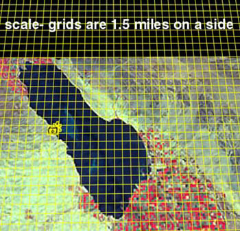
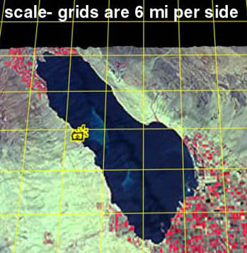
In order to determine the area of the Salton Sea, we will use the following images, which are gridded and scaled. The area is determined by counting the number of squares that include the image of the Salton Sea. for purposes of counting, we will apply the following % rule:
If a box is 50% full, then we will count it. If the box is less than 50% full, we will not count it.
By using this rule, we can grasp that as the boxes get smaller and smaller we can get a more accurate estimate of the area of the Salton Sea.
This was one of the common techniques for estimating the areas in the past. Another technique was to cut out the image and weigh it against a standard measured area. Now computers have advanced software that can measure the area quite accurately by a simple scanning or tracing process, but underlying all these schemes is the process of integration.
|
In the first image, we count 8 boxes that apply to this rule. Each box is equivalent to a 36 square mile area. So based on this graph, we calcuate an approximation of 288 square miles. The actual area of the basin is 360 square miles. This gives us a 20% error. With Riemann sums, we can get a more accurate number when we decrease the size of our squares. |
|
|
|
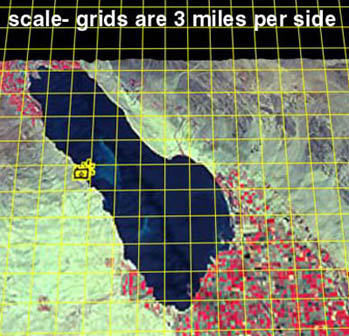
In the next graph, we count 33 boxes that apply to our 50% rule. Each box is equivalent to a 9 square mile area. So based on this graph, we calculate an approximation of 297 square miles. The actual area of the basin is 360 square miles. This gives us a 17.5% error. Since we can get a more accurate number when we decrease the size of our squares, we do it again. |
|
|
|
In the next graph, we count 137 boxes that apply to our 50% rule. Each box is equivalent to a 2.25 square mile area. So based on this graph, we calculate an approximation of 308.25 square miles. The actual area of the basin is 360 square miles. This gives us a 14% error. |
An integral computes the area under some arbitrary curve, given by a function.When a shape is complex, like our example of the Salton Sea, we can approximate the area by breaking up the region into smaller pieces whose areas are easily calculated, such as squares or rectangles.
Below we find the area under the curve of a cubic polynomial. One simple idea, developed by Riemann, was to split up the region into a collection of rectangles that closely approximate the area. The concept is to first divide the segment under the curve on the x-axis into some number of evenly spaced intervals. Then use the curve to find the height of the rectangle approximating the region under the curve. Since the area of a rectangle (length x width) is easily found, we can simply add the area of all the rectangles together to approximate the area under the curve. As is apparent in the example below, the approximation gets better as the width of the rectangles decrease. However, computationally this becomes harder with more rectangles to add together.
We examine how the process of Riemann sums works with the following cubic function between x = 0 and x = 5:
The actual area under the curve is 28.75. (We'll learn how to find this value in the next section.)
|
First, the region is divided into
five rectangles with width one and height taken to be the
midpoint in each interval. The red line is the plot
of the function Here we have 5 rectangles, which is a pretty coarse representation of the total area under the curve. Some of the area is not included, and some of the boxes stick out into where the curve shouldn't be counting area. The regions each have width 1, so the area is approximated by (f(1/2)+ f(3/2)+ f(5/2)+ f(7/2)+ f(9/2)) =
Evaluated, this gives us an approximate area of 28.125. This is 2.17% less than the actual area. |
 |
|
With 10 rectangles, the area is better calculated using this method, but you have to work a little harder. Now the widths of the rectangles are 0.5, so the area of the rectangles are (f(1/4)+ f(3/4)+ ...+ f(19/4))0.5 =
Evaluating this gives us an approximate area of 28.59375. This is 0.543% less than the actual area.
|
 |
|
With 20 rectangles, the approximating rectangles are even better. However, calculating the sum is very tedious without the help of the computer. Here the width is 1/4, so the sum of the areas is (f(1/8)+ f(3/8)+ ...+ f(39/8))(1/4) =
This now gives the approximate value of the region as 28.7109375. This is 0.135% less than the actual area.
|
 |
|
With 40 rectangles, there is a very dense grid of rectangles. To our eyes this is a very close match to the actual value of the area under the curve. With the help of a computer, the sum of the rectangles is performed very rapidly to give this increasingly accurate approximation to the area. In this case, the width of the rectangles are 1/8, so the Riemann sum becomes (f(1/16)+ f(3/16)+ ...+ f(79/16))(1/8) =
The approximate area is now given by 28.74023438. This is 0.034% less than the actual area. This process can be continued with the width of the rectangles becoming "infinitesimally small" as the mathematicians like to call it. In the limit, these Riemann sums appear to give the actual value to the area under the curve.
|
 |
|
Animation of the rectangles converging on the answer to the integral. |
 |
|
Click Here (for the maple worksheet that produced these graphics.) |
|
The example above illustrates the idea behind Riemann sums, where the area under a curve can be approximated by adding a collection of rectangular regions. As the width of the rectangles becomes smaller, the approximation of the area is better. In the limit with an infinite number of these rectangles with infinitesmally small widths, the Riemann sum should go to the actual area of the region.
As the example above illustrates, a good approximation to finding the area requires adding up a large number of thin rectangles. For convenience, we use summation notation to make these expressions easier to write and understand. For students who are unfamiliar with summation notation, it is actually quite simple. Say we want to add all the integers from 1 to 10, it could be written
However, summation notation gives the simpler form:

This notation is very important when you work in statistics with a large number of data points. Suppose you have 47 pieces of data, x1,..., x47, and wanted to find the average of these. The technique of finding the average is to add the numbers and divide by 47. Using summation notation, we can write the average, xave, as
Definition of Riemann Integral
Suppose that we want to find the area under some continuous function f(x) between x = a and x = b. As demonstrated by our example above, we want to divide the interval [a, b] into a large number of very small intervals. For simplicity of discussion, we will divide the interval into n even intervals (though Riemann sums do not require this restriction). Also, for simplicity, we will always evaluate the function, f(x), at the midpoint of any subinterval.
Let x0 = a and xn = b. Define Dx = (b - a)/n and xi = a + i Dx for i = 0,...,n. We can see that the numbers xi are evenly spaced along the interval [a, b]. This is partitioning the interval [a, b] into n subintervals [xi-1, xi] each with length Dx. The midpoint of each of these intervals is given by ci = (xi + xi-1)/2. In our example above, we found the height of the approximating rectangle by evaluating the function at the midpoint, ci. Thus, the area of the rectangle, Ri, over the interval [xi-1, xi] is given by its height times its width or
A figure showing this rectangle in reference to the complete region we are studying is shown in the diagram below.
To find the area under our continuous function f(x) between x = a and x = b, we need to add up all of the areas of all of the rectangles, Ri. With the summation notation developed above, we have the formula
The specific formula we have developed above is known as the Midpoint Rule for Integration. It is a valuable numerical method for approximating integrals that cannot be computed exactly. (However, like Euler's formula for differential equations, there are much better numerical methods for integration.) Below is a diagram showing the Midpoint Rule using the areas of the rectangles discussed above.
The Midpoint Rule described above is a specialized form of Riemann sums. The more general form of Riemann sums allows the subintervals to have varying lengths, Dxi. In addition, The choice of where the function is evaluated need not be at the midpoint as described above. The Riemann integral is defined using a limiting process, similar to the one described above.
Definition of Riemann Integral: Let f(x) be a continuous function in the interval [a, b]. Partition the interval [a, b] into n subintervals [xi-1, xi]. Assume that Dxk is the largest of these subintervals. Let ci be some point in the subinterval [xi-1, xi]. The nth Riemann sum is given by
and the Riemann integral is defined by
Numerical Methods for Integration
As noted in the beginning of the section on differential equations, there many differential equations that cannot be solved exactly. This is also the case for many integrals. However, when an integral is defined over a specific interval, as stated above for the Riemann integral, then there are a number of methods for finding approximate solutions to the integral. The Riemann integral defined above was shown to represent the area under a function on a specified interval. This integral is called a definite integral and is written:

The numerical methods approximate this definite integral in several ways.
Midpoint Rule: As noted above, the midpoint rule is a special case of Riemann sums where the interval integration [a, b] is divided n subintervals [xi-1, xi] each with length Dx = (b - a)/n. The endpoints are given by x0 = a and xn = b. The midpoint of each of these intervals is specified by ci = (xi + xi-1)/2, and the function is evaluated at this midpoint to given the height of each approximating rectangle, f(ci). The midpoint rule approximates the definite integral by adding the areas of the n rectangles. The formula is given by
This is the formula used above to motivate the definition of the Riemann sum and is simply a special case of the Riemann sum.
Trapezoid Rule: The trapzoid rule is an alternate method of numerically approximating the area under a curve and can be visualized in the figure below. The technique begins like the midpoint rule where the interval integration [a, b] is divided n subintervals [xi-1, xi] each with length Dx = (b - a)/n and the endpoints are given by x0 = a and xn = b. However, instead of evaluating the function at the midpoints of the subintervals, the function is evaluated at each of the endpoints of the subintervals, which makes this technique much better when applied to real data. A line segment is formed between these function evaluations on each subinterval, and the area of the resulting trapezoid is computed. (There is an exercise to remind you how to find the area of a trazezoid in case you have forgotten.) The trapezoid rule approximates the definite integral by adding the areas of the n trapezoids. The formula is given by
The formula has a similar accuracy to the midpoint rule. It is slightly more complicated in form, but has the advantage of performing the function evaluations at the endpoints of the intervals.
The figure below illustrates the Trapezoid rule using the same function as above and 5 subintervals. The function is shown in blue, while the trapezoid approximations are the green trapezoids.

In the figure above, we use the function
f(x) = x3 - 6x2 + 9x + 2
which was illustrated above for the Midpoint rule in developing the Riemann sums. For the Trapezoid rule dividing the interval [0, 5] into 5 subintervals, the integral approximation becomes
Comparing this to the actual integral value of 28.75 gives an approximation that is 4.3% too high, which is a similar error to the midpoint rule shown above.
Example 1: Use the Midpoint rule and the Trapezoid rule to approximate the integral of
f(x) = x2
for x in the interval [0,2] with n = 2 and n = 4.
Solution: For n = 2, the two subintervals are [0,1] and [1,2], and the value of Dx is 1.
For the Midpoint rule, the midpoints are c1 = 1/2, so f(1/2) = 1/4, and c2 = 3/2, so f(3/2) = 9/4. The Midpoint rule gives
For the Trapezoid rule, the integral approximation formula gives
For n = 4, the four subintervals are [0,1/2], [1/2,1], [1,3/2], and [3/2,2], and the value of Dx is 1/2.
For the Midpoint rule, the midpoints are c1 = 1/4, so f(1/4) = 1/16, c2 = 3/4, so f(3/4) = 9/16, c3 = 5/4, so f(5/4) = 25/16, and c4 = 7/4, so f(7/4) = 49/16. The Midpoint rule gives
For the Trapezoid rule, the integral approximation formula gives
We will see in the next section that the actual value is given by

In each of the cases above, we see that the midpoint rule is under estimating the integral and the trapezoid rule is over estimating the value.
Simpson's Rule: The midpoint and trapezoid rules are very simple to grasp conceptually, and their formulae are relatively simple. However, neither form is very accurate, requiring a fairly large value of n to obtain a good approximation to the integral. Simpson's rule use more advanced mathematical ideas to obtain a much more accurate approximation to the integral without having a significantly more complicated formula for obtaining the approximation.
Simpson's rule approximates the function f(x) by quadratics. As in the previous approximation methods, the interval integration [a, b] is divided n subintervals [xi-1, xi] each with length Dx = (b - a)/n and the endpoints are given by x0 = a and xn = b. However, in this case, n must be an even integer. The formula for Simpson's rule is given by
This formula has significantly better accuracy than either the midpoint rule or trapezoid rule. Yet it is not significantly more complicated in its formula for calculating the approximate integral.
Example 2: Use the Simpson's rule to approximate the integral of
f(x) = x2
for x in the interval [0,2] with n = 2 and n = 4. Note that n is even in both cases as required for this approximation.
Solution: For n = 2, the two subintervals are [0,1] and [1,2], and the value of Dx is 1. Applying Simpson's rule we have
For n = 4, the four subintervals are [0,1/2], [1/2,1], [1,3/2], and [3/2,2], and the value of Dx is 1/2. Applying Simpson's rule we have
Note that in both of these cases, Simpson's rule gives the exact answer. This is because the approximation that is being done is a quadratic approximation to the quadratic function f(x) = x2.
More examples are provided in the Worked Examples section.
![[Maple Math]](images/rsums6.gif)
![[Maple Math]](images/rsums9.gif)
![[Maple Math]](images/rsums12.gif)
![[Maple Math]](images/rsums15.gif)