6.3. Population Simulation Example: One simulation
Note
This is based one one of the 100 recipes of the IPython Cookbook, the definitive guide to high-performance scientific computing and data science in Python.
The goal of this section is to present a fairly intuitive
example of how numpy arrays function
to improve the efficiency of numerical calculations.
The example involes a simulation of something
called a Markov process and does not require
very much mathematical background.
We consider a population with a maximum of  individuals and equal probabilities of
birth and death for any given individual:
individuals and equal probabilities of
birth and death for any given individual:
import numpy as np
P = 100  # maximum population size
a = .005  # birth rate
b = .005  # death rate
We simulate fluctuation in the population size over T moments in time
with a Markov chain of length T.
Each state in the chain represents a population size at a moment in time.
We represent this with a numpy vector x.
The vector x will contain the entire history
of population sizes.
We first set the population size
at time  to
to  .
.
T = 1000
x = np.zeros(T)
x[0] = 25
x[:20]
array([ 25.,   0.,   0.,   0.,   0.,   0.,   0.,   0.,   0.,   0.,   0.,
         0.,   0.,   0.,   0.,   0.,   0.,   0.,   0.,   0.])
We now simulate our chain. At each time step  , there is a
new birth with probability
, there is a
new birth with probability ![a \cdot x[t]](../_images/math/7e3478fd86662ef38ffd73709dac41978d99a8c5.png) , and independently,
there is a new death with probability
, and independently,
there is a new death with probability ![b \cdot x[t]](../_images/math/b0ffc7a86b41af52bfa753452e5a1c5d138ae8f3.png) . These
probabilities are proportional to the size of the population at that
time. If the population size reaches
. These
probabilities are proportional to the size of the population at that
time. If the population size reaches  or
or  , the
evolution stops.
, the
evolution stops.
for t in range(T - 1):
    if 0 < x[t] < P-1:
        # Is there a birth?
        birth = np.random.rand() <= a*x[t]
        # Is there a death?
        death = np.random.rand() <= b*x[t]
        # We update the population size.
        x[t+1] = x[t] + 1*birth - 1*death
    # The evolution stops if we reach $0$ or $N$.
    else:
        x[t+1] = x[t]
x[:25]
array([ 25.,  25.,  25.,  25.,  26.,  27.,  27.,  28.,  28.,  29.,  30.,
        30.,  30.,  31.,  31.,  31.,  31.,  31.,  31.,  31.,  32.,  32.,
        32.,  32.,  32.])
x[-25:]
array([  8.,   8.,   8.,   8.,   8.,   8.,   8.,   9.,   9.,   9.,   9.,
         9.,   9.,   9.,   9.,   9.,   9.,   9.,   9.,   9.,   9.,  10.,
        10.,  10.,  10.])
x[t]
10.0
We plot the evolution of the population size.
plt.figure(figsize=(6,3));
plt.plot(x);
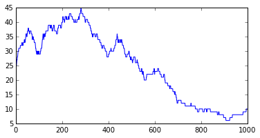
We see that, at every time, the population size can stay stable, increase by 1, or decrease by 1. This is a very jagged plot with day by day discrete variation (+ or - 1). The associated notebook shows how to smooth the plot using rolling means, but even the smoothed plots misses some very important properties of this trivial Markov model, as we will see in the next section.
6.4. Population Simulation Example: Using numpy for multiple simulations
Now, we now show how to simulate many independent trials of the
same Markov chain.
The vector
x will now contain
the population size of 100 independent trials
at a particular time.
To initialize x, the population sizes are set to random
numbers between and the maximum population size  .
.
We could run the previous simulation with a loop, but it would be
very slow (two nested for loops). Instead, we vectorize the
simulation by considering all independent trials at once.
As before, we need to loop over moments in time,
but at each time step, we update 100 trials
simultaneously with vectorized operations.
We initialize the ntrials=100 different trials with
a vector of size 100 with a randomly chosen initial population
size for each trial.
ntrials, P  = 100, 100
x = np.random.randint(size=ntrials,
                      low=0, high=P)
x
array([42, 12, 43, 41, 98, 11, 10, 21, 61, 12, 18, 10, 30, 31, 66,  7, 92,
       74, 89, 27, 62, 22, 22, 64, 93, 53, 14,  4, 79, 63, 29, 12, 98, 33,
       47,  5, 30, 99, 49, 35,  2, 52, 93, 41, 14, 29, 93, 78, 43, 27, 91,
       71, 43, 69, 75, 17, 61, 32, 71, 10, 72, 47, 40, 16,  1, 30, 86, 66,
       6, 56, 29, 14, 58, 69, 48, 53, 98, 79, 56, 95, 77, 10, 81,  9, 32,
       87, 14, 24, 44, 40, 12,  7, 45, 65, 17,  3, 17, 79,  7, 86])
Call this our trial vector.
As a illustration of what’s to come,
lets’s test to see that each trial in the trial
vector has a population size eligible for growth
> 0 and < P - 1. Notice how the Boolean test
is vectorized: It applies to each element of the trial vector and the
result is a vector of Booleans.
upd = (0 < x) & (x < P - 1)
array([ True,  True,  True,  True,  True,  True,  True,  True,  True,
        True,  True,  True,  True,  True,  True,  True,  True,  True,
        True,  True,  True,  True,  True,  True,  True,  True,  True,
        True,  True,  True,  True,  True,  True,  True,  True,  True,
        True,  True,  True,  True,  True,  True,  True,  True,  True,
        True,  True,  True,  True,  True,  True,  True,  True,  True,
        True,  True,  True,  True,  True,  True,  True,  True,  True,
        True,  True,  True,  True,  True,  True,  True,  True,  True,
        True,  True,  True,  True,  True, False,  True,  True,  True,
        True,  True,  True,  True,  True,  True,  True,  True,  True,
        True,  True,  True,  True,  True,  True,  True,  True,  True,  True], dtype=bool)
Note there is one False result, because the 38th element of
x was 99.
We can use such a Boolean vector to do a selective
update that changes (adds 1 to) only those trials in x
that are eligible for change.
x[upd] += np.ones(len(x[upd]))
array([43, 13, 44, 42, 99, 12, 11, 22, 62, 13, 19, 11, 31, 32, 67,  8, 93,
       75, 90, 28, 63, 23, 23, 65, 94, 54, 15,  5, 80, 64, 30, 13, 99, 34,
       48,  6, 31, 99, 50, 36,  3, 53, 94, 42, 15, 30, 94, 79, 44, 28, 92,
       72, 44, 70, 76, 18, 62, 33, 72, 11, 73, 48, 41, 17,  2, 31, 87, 67,
       7, 57, 30, 15, 59, 70, 49, 54, 99, 80, 57, 96, 78, 11, 82, 10, 33,
       88, 15, 25, 45, 41, 13,  8, 46, 66, 18,  4, 18, 80,  8, 87])
Note that every cell except the cell with value 99 has
been updated. WE will use a slight variation on this
idea in the code below.
The simulation function will work as follows.
We create a vector of size ntrials, with each cell containing
a randomly chosen number between 0 and 1. The probability of
at least one birth is a*x, and for each trial, we
we generate a birth only if the randomly chosen number
is less than a*x. Again, we do this in one line,
with a vectorized Boolean test on a vector of randomly
chosen numbers.
Z = (np.random.rand(ntrials) <= a*x)
Z
array([False, False, False, False, False, False, False, False, False,
       False, False, False, False, False, False, False, False,  True,
       True, False,  True, False, False, False, False, False, False,
       False,  True, False, False, False,  True, False, False, False,
       True,  True,  True, False, False, False, False,  True, False,
       False, False, False, False, False, False, False, False, False,
       False, False, False, False,  True, False, False, False, False,
       False, False, False,  True,  True,  True, False, False,  True,
       False, False, False, False,  True, False, False,  True,  True,
       False,  True, False, False,  True, False, False,  True,  True,
       False, False, False,  True, False, False, False, False, False,  True], dtype=bool)
Call Z the decision vector..
It will be convenient to swith from Booleans to 1’s and 0s, Again
we can do this a single vectorized operation on the decision vector Z.
1 * Z
array([0, 0, 0, 0, 0, 0, 0, 0, 0, 0, 0, 0, 0, 0, 0, 0, 0, 1, 1, 0, 1, 0, 0,
       0, 0, 0, 0, 0, 1, 0, 0, 0, 1, 0, 0, 0, 1, 1, 1, 0, 0, 0, 0, 1, 0, 0,
       0, 0, 0, 0, 0, 0, 0, 0, 0, 0, 0, 0, 1, 0, 0, 0, 0, 0, 0, 0, 1, 1, 1,
       0, 0, 1, 0, 0, 0, 0, 1, 0, 0, 1, 1, 0, 1, 0, 0, 1, 0, 0, 1, 1, 0, 0,
       0, 1, 0, 0, 0, 0, 0, 1])
So if we add such a decision vector to the cells of the current population vector eigible for update, we simulate a birth wherever there is a 1; if we subtract it, we simulate a death. Next define a simulation function to use such randomly generated decision vectors to simulate births and deaths. At every time step, we find the births and death for each trial by generating a random decision vector, and we update the population sizes with vectorized addition and subtraction.
def simulate(x, T):
    """Run the simulation."""
    for _ in range(T - 1):
        # Which trials to update?
        upd = (0 < x) & (x < N-1)
        # In which trials do births occur?
        birth = 1*(np.random.rand(ntrials) <= a*x)
        # In which trials do deaths occur?
        death = 1*(np.random.rand(ntrials) <= b*x)
        # We update the population size for all trials.
        x[upd] += birth[upd] - death[upd]
Now, we will look at the histograms of the population size at different times. These histograms represent the probability distribution of the Markov chain, estimated with independent trials. This kind of simulation of a sequence of trials according to a given probability distribution is called a Monte Carlo simulation.
We are interested in seeing the distribution of population sizes over all the simulations, so we draw histograms showing the number of simulations exhibiting various population sizes. This means dividing the possible population size (0-100) into bins. We choose 25 bins.
bins = np.linspace(0, N, 25);
N,len(bins),bins
(100, 25, array([   0.        ,    4.16666667,    8.33333333,   12.5       ,
          16.66666667,   20.83333333,   25.        ,   29.16666667,
          33.33333333,   37.5       ,   41.66666667,   45.83333333,
          50.        ,   54.16666667,   58.33333333,   62.5       ,
          66.66666667,   70.83333333,   75.        ,   79.16666667,
          83.33333333,   87.5       ,   91.66666667,   95.83333333,  100.        ]))
We will also try running our 100 simulations for histories of different lengths, short, medium, and long, to probe what the long term outcomes of our Markov model are.
plt.figure(figsize=(12,3));
T_list = [10, 1000, 10000]
for i, T in enumerate(T_list):
    plt.subplot(1, len(T_list), i + 1);
    simulate(x, T)
    plt.hist(x, bins=bins);
    plt.xlabel("Population size");
    if i == 0:
        plt.ylabel("Histogram");
    plt.title("{0:d} time steps".format(T));
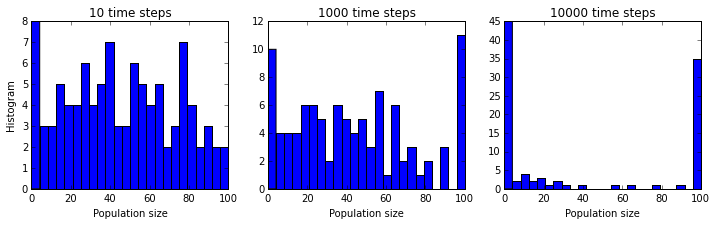
Now we can see a key property that was completely obscured
in the single simulation plot.
Whereas, initially, the population sizes look equally distributed
between and , they appear to converge to or
after a sufficiently long time. This is because the states
and are absorbing: once reached, the chain
cannot leave those states. Furthermore, these states can be reached from
any other state.
You’ll find all the explanations, figures, references, and much more in the book:
IPython Cookbook, by Cyrille Rossant, Packt Publishing, 2014 (500 pages).