|
|
Math 636 - Mathematical Modeling |
|
|---|---|---|
|
|
San Diego State University -- This page last updated 06-Oct-10 |
|
Lotka-Volterra Models
- Predator-Prey
- Lotka-Volterra model
- Equilibrium Analysis
- Linear Analysis
- Periodic Solutions
- Integrating about the Periodic Orbits
- Fitting the Parameters to the Model
- Model of Fishing
- Equilibria of the Fishing Model
- Worked Examples
- References
The previous section developed techniques for the qualitative analysis of nonlinear differential equations, where the differential equation contained a single unknown variable. The techniques allowed the reader to understand the behavior of mathematical models without actually solving the differential equations. This section looks at a predator-prey model where two species are involved. Thus, the differential equations describing the population dynamics must have two unknown variables, creating a system of differential equations. This system of differential equations cannot be solved exactly, so either numerical or qualitative methods need to be employed. One particularly interesting feature of this system is that the equilibrium analysis can give valuable ecological information, showing the use of pesticides is fundamentally a bad idea.
In this section, we develop the mathematical models for two species that are intertwined in a predator-prey or host-parasite relationship. As we have done before, the differential equations will be analyzed to find equilibria, linearize about the equilibria for stability analysis, show existence of periodic solutions, and perform some parameter identification to match the model to data. These techniques allow the reader to examine a wide range of models that have been developed in biology and other fields.
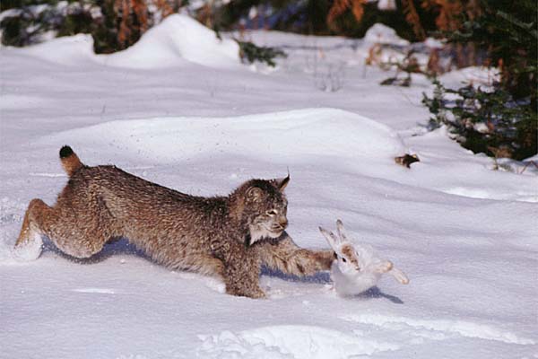
Our study begins with a classical example shown in many ecological textbooks, the population dynamics of a simple predator-prey system. Most mammalian predators rely on a variety of prey, which complicates mathematical modeling; however, a few predators have become highly specialized and seek almost exclusively a single prey species. An example of this simplified predator-prey interaction is seen in Canadian northern forests, where the populations of the lynx and the snowshoe hare are intertwined in a life and death struggle.
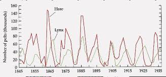
One reason that this particular system has been so extensively studied is that the Hudson Bay company kept careful records of all furs from the early 1800s into the 1900s. Below is a graph of the complete data set from 1845-1935. (This is a recreation of the data from MacLulich (1937) and was printed in the text by Purves et al (1992) and on the website of Wilensky and Riesmann.)
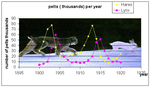
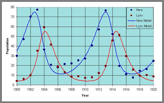
It is often assumed that the furs are representative of the populations in the wild because of the trapping intensity and trapping techniques, so these data can be used to represent the relative populations of the lynx and hares in the wild. The records for the furs collected by the Hudson Bay company showed distinct oscillations (approximately 12 year periods), suggesting that these species caused almost periodic fluctuations of each other's populations. Below is a graph of some of the fur data from the records of the Hudson Bay company (1900-1920).
We would like to create a mathematical model that explains these population fluctuations. Ecologists have predicted that in a simple predator-prey system that a rise in prey population is followed (with a lag) by a rise in the predator population. When the predator population is sufficiently high, then the prey population begins dropping. After the prey population falls, then the predator population falls, which allows the prey population to recover and completes one cycle of this interaction. Thus, we see that qualitatively oscillations occur. Can a mathematical model predict this? What causes cycles to slow or speed up? What affects the amplitude of the oscillation or do you expect to see the oscillations damp to a stable equilibrium? The models tend to ignore factors like climate and other complicating factors. How significant are these?
The Predator-Prey Model (Lotka-Volterra)
The mathematical predator-prey model and its cyclical nature was published in 1920 by Alfred Lotka, an American biologist and actuary, and developed throughout the 1920s, as an extension of Lotka's work in autocatalysis in chemical reactions. Lotka is regarded as the originator of many useful theories of stable populations, and his publications have been accepted as the basis for much subsequent work, including the Logistic model studied previously. Subsequent to these extensive publications, Vito Volterra in 1925 proposed the same model as an explanation of data from some fish studies of his son-in-law Humberto D'Ancona on the fishing industry in Italy (see below). Several of the two species predator-prey and competition models are called Lotka-Volterra Models, to distinguish them from other Lotka models in different fields of interest. Their models were natural extensions of the Verhulst or logistic model that we studied in earlier sections. This work is presented in most basic ecology textbooks and has many references on the web. One good study is shown in the work of M. Beals, L. Gross, and S. Harrell in their web modules from the University of Tennessee. Below we present the basic assumptions needed to create the classical Lotka-Volterra predator-prey model for the dynamics of the populations of a predator and its prey species.
Let H(t) be the population of snowshoe hares and L(t) be the population of lynx. As we have done before, we want to develop a mathematical model based on the growth rates for the populations. That is, the rate of change in a population is equal to the net increase (births) into the population minus the net decrease (deaths) of the population. We begin by applying this to the population of snowshoe hares. The rate of change of the hare population is dH/dt. The primary growth in the hare population is Malthusian, so this says that the population grows in proportion to its own population or a1H(t). We will make the simplifying assumption that the primary loss of hares is due to predation by lynx. Predation is often modeled by assuming random contact between the species in proportion to their populations with a fixed percentage of those contacts resulting in death of the prey species. Mathematically, this is given by a negative term, -a2H(t)L(t). Clearly, if there are other major predators or if the lynx population is low such that starvation due to overcrowding dominates the death rate, then alternative death terms would be more appropriate. Combining these terms, we obtain the growth model for the hare population:
Next we examine the population dynamics of the lynx. The rate of change of the lynx population is dL/dt. The primary growth for the lynx population depends on sufficient food for raising lynx kittens, which implies an adequate source of nutrients from predation on hares. Thus, the growth of the lynx population is similar to the death rate for the hare population with a different constant of proportionality. Mathematically, it follows that the growth of the lynx population can be written, b2H(t)L(t). The loss of lynx is presumed to be a type of reverse Malthusian growth. That is, in the absence of hares, the lynx population declines in proportion to their own population, which mathematically is given by the negative modeling term, -b1L(t). Clearly, if the lynx diet used other animals or crowding factors from other predators and lynx were taken into account, then these terms would have to be significantly modified. The growth model for the lynx population combines these terms above to give the following:
Clearly, the growth equations above are caricatures of the true complicated dynamics of these two animals. The model ignores the role of climate variation and the interactions of other species, including human disturbance. Other significant factors that are ignored in this modeling effort are the ages of the animals and the spatial distribution. However, we would like to see if this basic model can give a qualitatively similar picture to the dynamics that are observed in the Hudson Bay company furs that are graphed above. The Lotka-Volterra model is given by the system composed of the two differential equations written above. Note that these differential equations are intertwined into a system of differential equations with each growth model depending on the unknown variable (population) of the other.
As in previous analyses of dynamical systems, the first step to a qualitative analysis is finding the equilibria of the model. Equilibrium solutions are ones that do not change in time, so the derivatives are equal to zero. Thus, for the predator prey model above, we set
This results in a system of nonlinear algebraic equations to solve. If we let He and Le be the equilibrium solutions for the snowshoe hare and lynx populations respectively, then the system of algebraic equations that we need to solve is given by
In general, the solution of a system of nonlinear equations can be very difficult, but this case is relatively simple to solve using standard tools from algebra. These two equations can be factored, which aids in finding the solution. The first equation can be written
which implies that either He = 0 or a1 - a2Le = 0. Thus, we have possible equilibria at
Similarly, the second equation can be factored to give
which implies that either Le = 0 or -b1 + b2He = 0. Thus, we have possible equilibria at
The simultaneous solution of these two equations shows that when He = 0, then Le = 0, which gives rise to the trivial solution (extinction of both species)
The other equilibrium is given by
Unfortunately, the equilibria do not help explain the oscillatory behavior of the data reflected in the lynx and snowshoe hare data. We need information about the stability of these equilibria and further numerical and qualitative analysis techniques before we can demonstrate that this is an appropriate model. We perform a linear analysis and integrate about the equilibria, then return to the original example of Vito Volterra to show how even the equilibrium analysis of this simple model can explain some important ideas in population dynamics of a predator prey system.
As we showed in our previous work, a system of differential equations is linearized about its equilibria by finding the Jacobian of the vector function of the nonlinear system of differential equations. For the predator-prey model given above, the Jacobian matrix is given by
When this is evaluated about the equilibrium (He, Le) = (0, 0), the Jacobian matrix is
This has the eigenvalues and associated eigenvectors,
This shows that the equilibrium (0, 0) is a saddle node with solutions exponentially growing along the H-axis and decaying along the L-axis. The linear solution has the form
When this is evaluated about the equilibrium (He, Le) = (b1/b2, a1/a2), the Jacobian matrix is
This has the purely imaginary eigenvalues,
![]()
This shows that the equilibrium (b1/b2, a1/a2) is a center, which suggests that the solution cycles around as we suspected for the predator-prey model. The linear solution can be shown to satisfy
This produces a structurally unstable model. The model is structurally unstable because small perturbations from the nonlinear terms could result in the solution either spiraling toward or away from the equilibirum.
This model can be shown to have limit cycles for all positive initial conditions. The technique uses a simple integration following separation of variables of the differential equation found by dividing the two equations, i.e.,
The solution of this equation has the implicit solution
![]()
We need to demonstrate that this implicit solution has periodic solutions. Define the two sides of the implicit solution by
![]()
For the equation FH(H), we see that there is a vertical asymptote at H = 0. Differentiating this function gives
![]()
This has a minimum at the equilibrium He = b1/b2, then increases monotonically toward infinity. A similar argument shows that FL(L) has a maximum at Le = a1/a2, while the function begins with FL(0) = 0, then following the maximum asymptotically approaches 0. Graphs of these functions are shown below using the best model fit for the lynx-hare data.
The implicit solution shows that these functions are equal (with FL(L) shifting depending on the integration constant). Based on the analysis and the graphs, then they can be equal only on the range between the minimum of FH(H) and the maximum of FL(L). When FH(H) is at the minimum, then FL(L) has two distinct possible values. These two values correspond to the high and low values of the lynx population in the periodic orbit. (See the points marked A and B below and on the graphs above.) As we consider larger values of FH(H), there are two values of H corresponding to each value of FH(H), and each of these two values of H are paired with two values of L until we reach the maximum of FL(L). At the maximum of FL(L), Le = a1/a2 and FH(H) has two distinct possible values, which correspond to the high and low values of the hare population in the periodic orbit. (See the points marked C and D below and on the graphs above.) It follows that there must be a periodic orbit.
Integrating about the Periodic Orbits
With the knowledge that the orbits are periodic, we can ask about the average value of the solution. Suppose that a particular orbit has a period of T. The average population of hares for one period is given by the integral
and the lynx average satisfies
Consider the differential equation for the hare population. If we divide by H(t), then integrate around one period we have the following:
Fitting the Parameters to the Model
As we did in the competition models before, we would like to find the least squares best fit to the data from the Hudson Bay company on the pelts of the lynx and hares. Below we present the table of data.
|
Year
|
Hares (x1000)
|
Lynx (x1000)
|
Year
|
Hares (x1000)
|
Lynx (x1000)
|
|
1900
|
30
|
4
|
1911
|
40.3
|
8
|
|
1901
|
47.2
|
6.1
|
1912
|
57
|
12.3
|
|
1902
|
70.2
|
9.8
|
1913
|
76.6
|
19.5
|
|
1903
|
77.4
|
35.2
|
1914
|
52.3
|
45.7
|
|
1904
|
36.3
|
59.4
|
1915
|
19.5
|
51.1
|
|
1905
|
20.6
|
41.7
|
1916
|
11.2
|
29.7
|
|
1906
|
18.1
|
19
|
1917
|
7.6
|
15.8
|
|
1907
|
21.4
|
13
|
1918
|
14.6
|
9.7
|
|
1908
|
22
|
8.3
|
1919
|
16.2
|
10.1
|
|
1909
|
25.4
|
9.1
|
1920
|
24.7
|
8.6
|
|
1910
|
27.1
|
7.4
|
To perform the least squares best fit to the data using the predator-prey model, we need good estimates of the parameters. The parameters that are varied for this model are the initial conditions, H(0) and L(0), and all of the growth and death rate constants, a1, a2, b1, and b2. The initial choices for the initial conditions come directly from the data, so we take
H(0) = 30 and L(0) = 4.
To find the rate constants, we use a number of the relations derived above. Recall that the integral about one period of the model gives the values of the equilibria. So if we average the data between two maxima or minima, then we should obtain a reasonable estimate of the equilibria for these data. Averaging the data between 1903 and 1913 (omitting the last year to not bias the maximum) for the hares and the data from 1904 to 1915 (again omitting 1915), we have the following equilibrium estimates
He = b1/b2 = 34.6 and Le = a1/a2 = 22.1.
The data indicate that the period of the solution should be around 12 years so from the eigenvalues of the equilibrium, we can get an estimate of the frequency
Note that this value is likely to be a little low because the period of oscillation generally increases as you move away from the equilibrium. This estimate is near the equilibrium, so using the higher value of the period, 12, generated a distance away from the equilibrium indicates that the product a1b1 is too low. From the model, we would expect that when the predator population is very low, then the prey population is undergoing Malthusian growth, so provides some estimate of the growth parameter a1. From the graph of the data, we see a low in lynx around 1910. At this time we see the hare population growing rapidly. If we use the population of 27.1 in 1910 and 40.3 in 1911, then assuming a Malthusian growth model of the form
![]()
we obtain the estimate
a1 =ln(40.3/27.1) = 0.397.
This estimate is clearly a little low because of the effects of predation that are ignored. Similarly, we examine the data for low populations of hares to find the exponential decline of the lynx population. We see that the steepest decline of the of the lynx population occurs between 1905 and 1906 with populations of 41.7 and 19, respectively. If we consider a decaying solution of the form
![]()
then the data gives the following estimate
b1 = ln(41.7/19) = 0.786.
Because of the growth term, the estimate above is should be low. Note that these estimates are reasonably consistent.
Combining the information above, we obtain the following initial estimates for the parameters
a1 = 0.4, a2 = 0.018, b1 = 0.8, and b2 = 0.023.
With these estimates on the parameters, we can use MatLab to find the least squares best fit of the model to the data. The MatLab code is given below as a single function.
function exitflag = lynx_hare
%Enter the data and the initial guess.
td = [0:20];
hare = [30 47.2 70.2 77.4 36.3 20.6 18.1 21.4 22 25.4 27.1 40.3 57 76.6 52.3
19.5 11.2 7.6 14.6 16.2 24.7];
lynx = [4 6.1 9.8 35.2 59.4 41.7 19 13 8.3 9.1 7.4 8 12.3 19.5 45.7 51.1 29.7
15.8 9.7 10.1 8.6];
p = [30 4 0.4 0.018 0.8 0.023];
%Finally we use the fminsearch routine as follows:
[p,fval,exitflag] = fminsearch(@leastcomp,p,[],td,hare,lynx);
p
fval
function J = leastcomp(p,tdata,xdata,ydata)
%Create the least squares error function to be minimized.
n1 = length(tdata);
[t,y] = ode23(@lotvol,tdata,[p(1),p(2)],[],p(3),p(4),p(5),p(6));
errx = y(:,1)-xdata(1:n1)';
erry = y(:,2)-ydata(1:n1)';
J = errx'*errx + erry'*erry;
function dydt = lotvol(t,y,a1,a2,b1,b2)
% Predator and Prey Model
tmp1 = a1*y(1) - a2*y(1)*y(2);
tmp2 = -b1*y(2) + b2*y(1)*y(2);
dydt = [tmp1; tmp2];
The output of this function gives the best parameter values as
H(0) = 34.91 and L(0) = 3.857
and
a1 = 0.4807, a2 = 0.02482, b1 = 0.9272, and b2 = 0.02756
with the sum of squares error being
J = 593.28.
We can graph the data and the model using these parameters and obtain the following graph of the populations of lynx and hares as functions of the year:
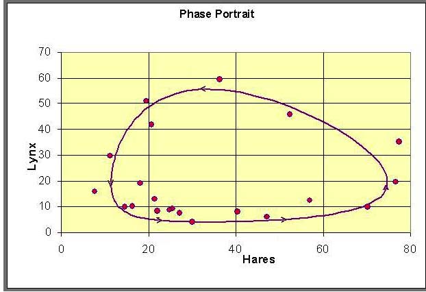
Similarly, we can plot the data with the periodic orbit to obtain a phase portrait.
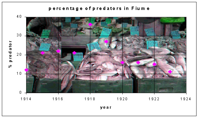
Humberto D'Ancona was an Italian biologist who, in 1924, completed a statistical study of fish populations in the Adriadic Sea. He observed that, during the time of reduced fishing in World War I, his populations showed an increasing percentage of predator fish, especially sharks and skates (or a decrease of prey fish). This increase in population of the predator fish declined after the war. Vito Volterra, his father-in-law, was an Italian mathematician who had recently retired, and D'Ancona asked Volterra if there was a mathematical model which could explain this observed relative change in the populations of fish species. Within a couple of months, Volterra produced a series of mathematical models for the interaction of two or more species. Below is a table showing his data with a graph.Why should World War I affect the relative frequency of fish in Italian ports?
|
1914
|
1915
|
1916
|
1917
|
1918
|
1919
|
1920
|
1921
|
1922
|
1923
|
|
12 |
21 |
22 |
21 |
36 |
27 |
16 |
16 |
15 |
11 |
|
|
|||||||||
D'Ancona asked his father-in-law Vito Volterra, a famous Italian mathematician, if there was a mathematical model that could explain the increase in predator fish during the World War I period. Within a couple of months, Volterra produced a series of models for the interaction of two or more species.
The data above do not show oscillations, but there is clearly a rise and fall of the percent of sharks and skates in the fish catch due to effects of the war. A slight modification of the predator prey model developed above and an equilibrium analysis can be used to explain the observed data. Volterra reasoned that the change in the relative frequency must be related to the changes in the fishing practices during the war. In particular, because of the dangers of fishing during wartime and because of the loss of fishermen who were required to fight in the war, there was a significant decline in the amount of fishing during the war. This needs to be included in the mathematical model for the interaction between the predatory fish and their prey fish.
Let F(t) be the food fish or prey fish and S(t) be the shark and skate population (less desirable catch in those times). The Lotka-Volterra predator-prey model, which includes fishing can be written:
The terms with the coefficients a1, a2, b1, and b2 are the same as were developed for the predator-prey model for the lynx and hares above. There is another significant predator to both of these populations, human fishermen. The fishermen trolled for these fish primarily with nets that indiscriminately extracted both food fish and the predatory fish (though possibly at different rates). To model the effects of fishing, we add the terms a3F and b3S, where a3 and b3 reflect the intensity of fishing. These terms are appropriate as an approximation, since the fishing nets will sweep out a percentage of all fish in their paths that is proportional to the populations of fish in the region that is being fished.
Since the data that D'Ancona collected represent annual percentages of fish in the markets, one can assume that the populations of fish during that time are approximately in equilibrium. It can be shown (mathematically) that the average population about a cycle of the Lotka-Volterra model is its equilibrium value. Thus, if the fishing populations are cycling less than annually, the annual catch should reflect the equilibrium population. So this model is assuming a more rapid dynamics of the fish population than the lynx and hares above. If Fe and Se represent the equilibrium populations of the food fish and sharks/skates populations respectively, then these equilibria are found by solving
As before, these equations are factored to make solving them easy. The first equation is written
which implies that either Fe = 0 or a1 - a2Se - a3 = 0. Thus, the equilibria have either
 .
.Similarly, the second equation is factored to form the equation
which implies that either Se = 0 or -b1 + b2Fe - b3 = 0. Thus, we have possible equilibria at
 .
.Thus, as before, one of the equilibria is the trivial solution with neither species existing,
The other equilibrium satisfies
 .
.which agrees with the equilibrium of the lynx-hare model above. This equilibrium value is fixed and independent of human interaction. It is determined solely by the ecological interactions of the fish and their predators, the sharks and skates. The human fishing activity is reflected in the parameters a3 and b3, which are both positive. As the level of fishing increases, these parameters increase. From the analysis above, we saw that the nonzero equilibrium is given by
The equilibrium value of the food fish, Fe, clearly increases as b3 increases. In one respect, this makes sense because one would expect the food fish to benefit from the harvesting by humans of their natural predators in the Adriadic Sea. However, the model shows that human interference (at least when not too extreme) by harvesting the food fish, which is reflected in the constant a3, does not appear in the formula for Fe, and so has no effect on the food fish equilibrium. This result is not so intuitive!
Similarly, the equilibrium value of the sharks and skates, Se, clearly decreases as a3 increases. This makes sense because the fisherman are in direct competition with the sharks and skates for this food source. However, again the model shows that human interference (at least when not too extreme) by harvesting the sharks and skates, which is reflected in the constant b3, has no effect on the shark and skate equilibrium. Once again, this result is not so intuitive!
The data of D'Ancona agrees qualitatively with our equilibrium analysis. During World War I, the fishing fleets would be less likely to go out. This implies that the level of fishing decreases, so a3 and b3 decrease. Thus, the equilibrium value for the food fish decreases, while the equilibrium for the sharks and skates increases.The result appearing in the market data would be an increase in the percentage of shark and skates available, which is shown in the data. Because of this decrease in the level of fishing, the overall amount of fish products in the market would decrease, which is not shown in the data. There is insufficient data to obtain more than this gross qualitative overview of the effect of human fishing on the population dynamics. Detailed studies would be required to obtain more quantitative results and fit the six parameters in this system of differential equations.
[1] Lotka, A. J. 1920. Analytical note on certain rhythmic relations in organic systems, Proc. Natl. Acad. Sci. 6, 410-415.
[2] Lotka, A. J. 1925. Elements of Physical Biology. Baltimore: Williams & Wilkins Co.
[3] Volterra, V. 1926. Variazioni e fluttuazioni del numero d'individui in specie animali conviventi. Mem. R. Accad. Naz. dei Lincei. Ser. VI, vol. 2.