|
|
Math 636 - Mathematical Modeling |
|
|---|---|---|
|
|
San Diego State University -- This page last updated 16-Sep-09 |
|
|
|
Math 636 - Mathematical Modeling |
|
|---|---|---|
|
|
San Diego State University -- This page last updated 16-Sep-09 |
|
Influenza
Influenza or flu is a
viral infection that is readily transmitted through the air and causes
respiratory problems in humans and other animals. It occurs seasonally
and results in an average of 30,000 deaths in the U. S. annually
primarily among the young and old. There have been some epidemics, such
as the pandemic of 1918, which resulted in over 30 million deaths
around the world.
There are two primary types, A and B of influenza, which appear
seasonally, usually starting in the fall and continuing through the
winter months. These types mutate creating new strains each year. Flu
is an RNA virus with 11 genes that mutate regularly, making it
difficult to create general vaccines. Each year scientists anticipate
the most likely dominant strain and determine which mutant is most
likely to spread in order to create a vaccine to protect the
population. In addition to the many deaths, this disease results in
huge economic losses from lost work and treatment of fragile patients.
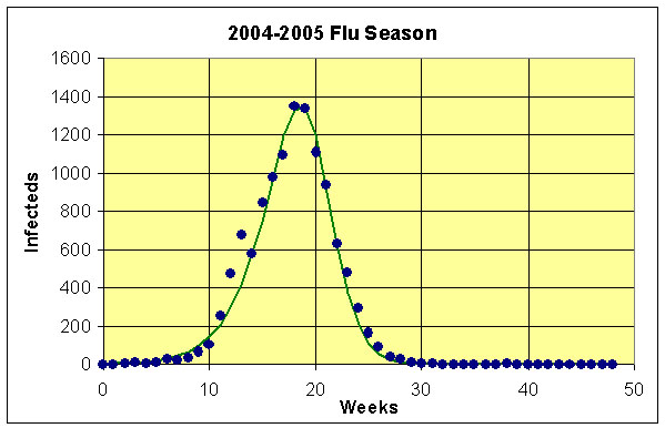
Below we provide data from the Center of Disease Control for one season of flu. The table below gives the number of cases week by week for a control set of individuals. In particular, we consider the data for the cases with Type A for the flu season in 2004 and 2005, where 99.7% of these cases were influenza A (H3N2) viruses. These data come from 157,759 samples that were tested amongst people exhibiting flu-like symptoms. The first week, n = 0, corresponds to the last week in September, which is near the seasonal start of the flu season in the U. S.
| n (wk) | In | n (wk) | In | n (wk) | In |
| 0 | 3 | 17 | 1096 | 34 | 2 |
| 1 | 2 | 18 | 1354 | 35 | 0 |
| 2 | 7 | 19 | 1335 | 36 | 2 |
| 3 | 12 | 20 | 1109 | 37 | 1 |
| 4 | 9 | 21 | 936 | 38 | 6 |
| 5 | 10 | 22 | 627 | 39 | 0 |
| 6 | 27 | 23 | 476 | 40 | 0 |
| 7 | 21 | 24 | 295 | 41 | 1 |
| 8 | 36 | 25 | 164 | 42 | 0 |
| 9 | 63 | 26 | 94 | 43 | 0 |
| 10 | 108 | 27 | 37 | 44 | 0 |
| 11 | 255 | 28 | 26 | 45 | 1 |
| 12 | 472 | 29 | 15 | 46 | 0 |
| 13 | 675 | 30 | 8 | 47 | 3 |
| 14 | 580 | 31 | 5 | 48 | 0 |
| 15 | 844 | 32 | 3 | ||
| 16 | 974 | 33 | 1 |
SIR Model for
Influenza
Influenza is a disease that follows a classic
mathematical model known as an SIR model. The population can be divided into susceptible,
infected, and recovered individuals. Once a person has a particular
strain of one of the types of the influenza virus, then that individual
develops immunity to that specific strain, preventing reinfection.
(This is why flu viruses need to mutate to keep finding new hosts.)
Since flu acts over a very short period of time, we will simplify our
model by assuming that the population remains constant with a size of N. This means that it is sufficient to simply
keep track of two classes of individuals, the susceptibles, Sn, and the infected, In, as the recovered satisfy
Since we are ignoring births and deaths in the population, we only
consider the spread of the disease, which is based on successful
contacts (such as inhaling aerosol infected particles from the sneeze
of an infected individual into the lungs of a susceptible host). The
discrete mathematical model is given by the system of equations:
Sn+1 = Sn - (b/N)SnIn,
In+1 = (1 - g)In + (b/N)SnIn,
where bS/N represents the proportion of contacts by an infected individual that result in the infection of a susceptible individual. The parameter g is the probability that an infected person recovers (enters class R of the SIR model). The ratio 1/g is the average length of the infectious period of the disease.
Modeling Assumptions
The SIR model above is a discrete dynamical system, where populations are exmined at discrete time steps. The model assumes that the population is well-mixed, so all individuals are equally likely to encounter other individuals. This probably works well for local populations, such as a particular school, but is not good for the entire U. S., where these data are collected. It is well known that there are significant regional outbreaks, and often containing regional outbreaks is key to controlling a disease.
The model also assumes that an individual becomes infectious as soon as he or she becomes infected, when in fact there are often time delays inherent in a disease. This factor is sometimes modeled with an SEIR model, where E represents exposed individuals. This simplistic model doesn't account for many factors that could prove important in the course of the disease, yet it gives some understanding of the disease and how we might affect its spread.
Modeling Simulation
We want to simulate the SIR model and try to fit it to the CDC data in the table above. Assume that the control population consists of N = 157,759, which is based on the number of samples that the CDC analyzed. This is obviously not representative of a well-mixed homogeneous population. However, it would be very difficult to obtain a good choice for N. With this assumption for our population, it becomes natural to take I0 = 3 and S0 = 157,756 = N - I0. We would like to simulate the model and determine the best values of the parameters, b and g, that match the data from the CDC data. These parameters are key to understanding the nature of a disease.
Epidemiologists often examine what is called the basic reproduction ratio given by
R0 = b/g,
which provides a measure of how rapidly a disease will spread and how much of the population will be affected by a particular disease. Also, the average length of the infectious period is equal to 1/g.
We simulate the model, finding the Least Sum of Square Errors (LSSE) by changing the parameters, b and g. The SSE is found between the CDC data on the infecteds and the model simulation of In. Using Excel's Solver, we obtain a LSSE = 155,083, and the best parameter values are:
b = 3.993 and g = 3.517.
The fit is seen below in the graph of the model and data. (See Excel Sheet.)
By taking the inverse of g, we find that the average duration of the infectious period is 1.99 days. The basic reproduction ratio is
R0 = 1.135.
To determine the impact of a particular flu season, we want to know the total number of individuals who were infected by the influenza virus. Since we are assuming a constant population N and because the number of infected individuals is essentially zero at the end of the simulation. We estimate the total number of cases of flu by computing the number in the recovered class, so
Rn = N - Sn = 39,001,
for n large. This represents approximately 24.7% of the population.
Controlling the Flu
The CDC is interested in minimizing the impact of flu on the
population, so uses a number of different controls. We examine three
different controls that are employed to fight outbreaks of the
flu.
The first line of defense, of which you are undoubtedly aware, is the
annual flu vaccine. The effect of a vaccine is to lower the population
of susceptible individuals, which is terms of our model is simply to
lower S0 by moving a number of individuals to R0. (In fact, many individuals already have
immunity to a given strain of the flu because of earlier contact with a
related strain.) Suppose we vaccinate 5% of the total population
at the very beginning of the flu season (assuming that the vaccine is
100% effective). This immediately shifts some of the population to the
recovered individuals in the model. We calculate the initial
susceptible population by
Assuming no other changes for this epidemic, then the values of g and b remain the same as above. We simulate the SIR model with this new initial condition. (See the graph below.) The effect is to delay the onset of the flu epidemic and dramatically reduce the number of people who become infected. The total number of people becoming infected is now
Rn = N - Sn = 22,311,
for n large. This represents approximately 14.1% of the population, so the number getting the flu about 60% of the number had there been no treatment.Rn = N - Sn = 23,483,
for n large. This represents approximately 14.9% of the population, so the number getting the flu again about 60% of the number had there been no treatment.Rn = N - Sn = 24,305,
for n large. This represents approximately 15.4% of the population, so the number getting the flu again about 60% of the number had there been no treatment. Thus, all of the proposed treatment options are similarly effective and significantly affect the outbreak of the flu epidemic.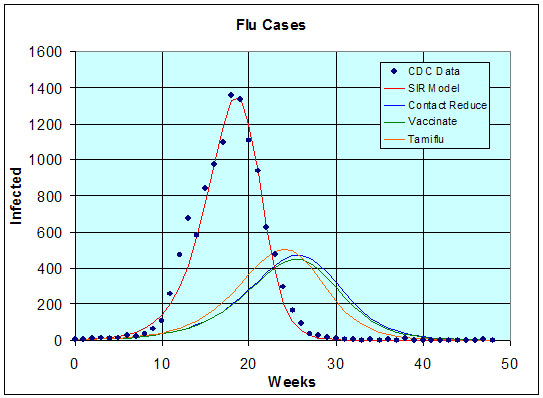
Compare and contrast the different
approaches to controlling a flu outbreak. Give advantages and
disadvantages of each of the controls. Include a discussion of the
practicality and financial burden of each of these approach. Give a
couple of strengths and weaknesses for this SIR model. Select another
disease that satisfies the SIR model and discuss how this lab applies
to treatment of the disease you are considering. How does this study
apply to elimination of other serious diseases?
Finding the Equilibria
We find equilibria by setting Sn+1 = Sn = Se and In+1 = In = Ie. When we substitute into the first equation, we find
Se = Se - (b/N)SeIe,
which yields
(b/N)SeIe = 0
Se = 0 or Ie = 0.
The second equation gives
Ie = (1 - g)Ie + (b/N)SeIe,
so
gIe = (b/N)SeIe.
If Se = 0, then necessarily Ie = 0. If Ie = 0, then Secan be anything. It follows that the equilibria are
Ie = 0 and 0 < Se < N.
Linearizing about the Equilibria
We quickly review the linearization of a system given by:
The Jacobian matrix is given by
The linearized system for the SIR model about the equilibrium (Se, Ie) = (Se, 0) is given by the linear discrete system:
Since this is an upper triangular matrix, the eigenvalues are given by the diagonal elements. One eigenvalue is l1 = 1, while the other eigenvalue satisfies
l2 = 1 - g + (b/N)Se.
For the equilibrium to be unstable and the disease to spread, we need l2 > 1 or 1 - g + (b/N)Sn > 1. Thus,
bSn/N > g
![]() .
.
We see that if R0 > 0 and Sn ~ N, then the disease will spread. However, as Sn gets smaller with more people establishing immunity, then N/Sn > b/g and the disease dies out.
References [1] CDC Flu website - www.cdc.gov/flu/ Specifically for
data: www.cdc.gov/flu/weekly/fluactivity.htm
(last visited Sept. 2009).
[2] Wikipedia - en.wikipedia.org/wiki/Influenza
(last visited Sept. 2009).